Ersoy O.K. Diffraction, Fourier optics, and imaging (Wiley, 2006)(ISBN 0471238163)(427s) PEo

208	HOLOGRAPHY

bðx; yÞ is related to the aberrations discussed in Section 13.5. Similar equations can be written at the hologram point ðx; yÞ relative to the origin for fcðx; yÞ, the phase due to the reconstruction wave at wavelength l2, and frðx; yÞ, the phase due to the recording reference wave at wavelength l1.

With respect to Eqs. (13.2-8) and (13.2-9), the important phase terms for U3 and U4 can be written as

fV ¼ fc þ fo fr	ð13:5-4Þ
fR ¼ fc fo þ fr	ð13:5-5Þ

At this point, terms of order higher than 1 in 1=z or 1=zc or 1=z0 are neglected. Writing fI for f3or f4, we get

2p 1

2p 1

fI ðx; yÞ ¼

ðx02 þ y02

2x0xr 2y0yrÞ þ

ðx2 þ y2 2xxo 2yyoÞ

l2

2zc

l1

2zo

2p 1

2

2

ðx

þ y

2xxr 2yyrÞ

ð13:5-6Þ

l1

2zr

where þ sign is for f3 and – sign is for f4.

The hologram magnification Mh is defined by

x0

y0

Mh ¼

¼

x

y

and the wavelength ratio is given by

m ¼

l2

l1

Then, Eq. (13.5-6) can be written as

1

m

m

2

ðx02 þ y02Þ

þ

3

zc

Mh2zo

Mh2zr

p

6

mxo

mxr

7

fI

ð

x; y

Þ ¼ l2

6

2x

zc

þ Mhzo

Mhzr

7

6

2y

7

6

m

m

7

6

yo

yr

7

4

5

6

yc

7

6

zc

þ

Mhzo

Mhzr

7

ð13:5-7Þ

ð13:5-8Þ

ð13:5-9Þ

Equation (13.5-9) can be interpreted as the phase corresponding to another spherical wave originating from the point ðxI ; yI ; zI Þ. The relevant phase for this wave within the Fresnel approximation is given by

fI0	p	ðx02 þ y02 2x0xI 2y0yI Þ
	¼ l2zI		ð13:5-10Þ

ANALYSIS OF HOLOGRAPHIC IMAGING

209

Setting f0I ¼ fI yields

	zI ¼	Mh2zczozr		ð13:5-11Þ
		Mh2zozr þ mzczr mzczo
	x	Mh2xczozr þ mMhxozczr mMhxrzczo		ð	13:5-12	Þ
		Mh2xczozr þ mzczr mzczo
	I ¼
	y	Mh2yczozr þ mMhyozczr mMhyrzczo		ð	13:5-13	Þ
		Mh2yczozr þ mzczr mzczo
	I ¼

Which image is virtual and which image is real is determined by the signs of zr and zc, respectively. The transverse magnification is given by

Mt ¼

qxI

¼

Mh

qxo

1 þ

M2z

o

zo

h

mzc

zr

Ma

qzI

Mh2

d

2

zo

3

¼ qzo ¼ m dzo

4

2

Mh2

1

5

61

zo

mzc

þ zr

7

6

7

1

M

h

¼

m

1 þ

Mh2zo

zo

2

mzc

zr

¼ m1 Mt2

ð13:5-14Þ

ð13:5-15Þ

EXAMPLE 13.2 Determine m so that Ma ¼ Mt in magnitude.

Solution: We set

jMaj ¼ m1 Mt2 ¼ Mt

Hence,

m ¼ Mt

ð13:5-16Þ

This means the changes in hologram size and the reference wave origin can be compensated by choosing a new wavelength satisfying Eq. (13.5-16). By the same token, if the wavelength is changed, the hologram size and/or the reference wave origin can be changed to make the two types of magnification equal to each other as much as possible.

210	HOLOGRAPHY

13.6ABERRATIONS

In discussing aberrations, it is more convenient to replace the rectangular coordinates x and y by the polar coordinates r and y. Wave front aberrations are defined by the phase difference fAðr; yÞ between the ideal spherical wave front and the actual wave front with source at ðxI ; yI ; zI Þ.

We will consider the aberrations of the image U3 due to the third-order terms as in Eq. (13.5-3). The third-order terms due to fc; fo; fr are combined to give the thirdorder term in the actual wave front. The aberration wave function becomes

				2		1	r4S			þ	1		r3ðCx cos y þ Cy sin yÞ											3
						8					2
			2p	6																				7
				6																				7
fA	r; y	Þ ¼ l2		6		1	r2	ð	Ax cos2 y							þ	Ay sin2 y			þ	2AxAy cos y sin y		Þ	7
ð				6		2	2				1													7
				6		1																		7
				4		4				þ	2			ð				þ				Þ		5
				6																				7
				6			r F							r	Dx cos y				Dy sin y					7

where the parameters belong to the following aberrations: S: spherical aberration

Cx, Cy: coma

Ax, Ay: astigmatism F: field curvature Dx, Dy: distortion

They are given by the following equations:

1

m

m

1

S ¼

þ

zc3

Mh4zo3

Mh4zr3

zI3

xc

mxo

mxr

xI

Cx

¼

þ

zc3

Mh3zo3

Mh3zr3

zI3

yc

myo

myr

yI

Cy

¼

þ

zc3

Mh3zo3

Mh3zr3

zI3

xc2

mxo2

mxr2

xI2

Ax

¼

þ

zc3

Mh2zo3

Mh2zr3

zI3

yc2

myo2

myr2

yI2

Ay

¼

þ

zc3

Mh2zo3

Mh2zr3

zI3

F

¼

xc2

þ yc2

mðxo2 þ yo2Þ

mðxr2 þ yr2Þ

xI2 þ yI2

zc3

Mh2zo3

þ

Mh2zr3

zI3

D

¼

xc3

þ xcyc2

mðxo3 þ xoyo2Þ

mðxr3 þ xryr2Þ

xI3

þ xI yI2

zI3

x

zc3

Mhzo3

þ

Mhzr3

D

¼

yc3

þ ycxc2

mðyo3 þ yoxo2Þ

mðyr3 þ yrxr2Þ

yI3

þ yI xI2

zI3

y

zc3

Mhzo3

þ

Mhzr3

ð13:6-1Þ

ð13:6-2Þ

ð13:6-3Þ

ð13:6-4Þ

ð13:6-5Þ

ð13:6-6Þ

ð13:6-7Þ

ð13:6-8Þ

ð13:6-9Þ

ABERRATIONS

211

EXAMPLE 13.3 Determine S, Cx, and Ax when the recording and reconstruction waves are plane waves.

Solution: In this case, zr and zc are infinite. Therefore S; cx, and Ax become

m

"

m2

#

S ¼

Mh4zo3

Mh2

1

Cx

m xc m xo

m2

1

xr m2

¼ Mh3zo2

"zc Mh zo

Mh2

! þ zr Mh2#

m

xo2

m

2

2m xo

xc mxr

2

Ax

1

xc mxr

¼ Mh2zo

"zo2

Mh2

zc þ Mhzr þ zc þ Mhzr #

! Mh zo

EXAMPLE 13.4 Determine Cx and Ax when zr ¼ zo

Solution: After a little algebra, we find

¼Mh

zo

Mh2zo2

zc2

þ zr

Mh2zo2 zc2

Cx

m

xo

1

1

xr

1

1

m

xo2

1

m

2 xo xc

mxr xr2 1

m

2 xc xr

Ax

¼Mh

zo2 Mhzo

þ Mhzc þ zc zo zc þ Mhzr þ zr2 Mhzo Mhzc zc zc zr

14

Apodization, Superresolution, and Recovery

of Missing Information

14.1INTRODUCTION

In optical imaging, diffraction is the major phenomenon limiting the resolving power of the system. For example, consider imaging of a distant star through a telescope. Because of the distance of the star, the image should form on the focal plane, ideally as a point. Instead, the image intensity is proportional to the square of the Fourier transform of the exit pupil of the telescope. As a result, the image consists of a central maximum in radiance surrounded by other optima (secondary maxima or minima) which may be mistaken for other sources. For the same reason, a second and weaker star nearby may be missed altogether.

The techniques of apodization and superresolution have the goal of minimizing the effects of finite aperture size. Superresolution is also closely related to the topic of recovery of missing information.

The algorithms discussed in this chapter are with discretized signals so that they can be directly implemented in the computer. The algorithms can also be easily converted to analog representation if so desired.

This chapter consists of eighteen sections. Section 14.2 is on apodization or windowing techniques. Various windowing sequences are highlighted in this section. Two-point resolution, which is inherent in optical imaging devices, and the general guidelines for the recovery of signals are covered in Section 14.3.

In succeeding sections, the basic theory needed to develop recovery algorithms is first described. Section 14.4 describes the basic theory for contractions and shows under what conditions iterations with a mapping transformation of vectors in a linear vector space leads to a fixed point. This is followed in Section 14.5 by an iterative method of contractions called the method of constrained iterative signal restoration for signal recovery. Section 14.5 follows up with the same theme in the case of deconvolution with a method called iterative constrained deconvolution.

Diffraction, Fourier Optics and Imaging, by Okan K. Ersoy

Copyright # 2007 John Wiley & Sons, Inc.

212

APODIZATION

213

A subset of contractions is projections which are introduced in Section 14.7. There are a number of different types of projections. The method of projections on to convex sets (POCS) is the one which is relatively easier to handle, and it is covered in Section 14.8. This method is further discussed in succeeding chapters as a tool which is used within other algorithms for the design of diffractive optical elements and other diffractive optical devices. In Section 14.9, the Gerchberg–Papoulis algorithm is discussed as a special case of the POCS algorithm in which the signal and Fourier domains are used together with certain convex sets. Section 14.10 gives other examples of POCS algorithms.

Two applications that have always been of major interest are restoration from phase and restoration from magnitude. The second application is usually much more difficult to deal with than the first application. An iterative optimization method for restoration from phase is discussed in Section 14.11. Recovery from a discretized phase function with the DFT is the topic of Section 14.12.

A more difficult type of projection is generalized projections in which constraints do not need to be convex. In such cases, iterative optimization may or may not lead to a solution. This topic is covered in Section 14.13. Restoration from magnitude, also called phase retrieval, can usually be formulated as a generalized projection problem. A particular iterative optimization approach for this purpose is discussed in Section 14.14.

The remaining sections discuss other types of algorithms for signal and image recovery. Section 14.15 highlights the method of least squares and the generalized inverse for image recovery. The singular value decomposition for the computation of the generalized inverse is described in Section 14.16. The steepest descent algorithm and the conjugate gradient method for the same purpose are covered in Sections 14.17 and 14.18, respectively.

14.2APODIZATION

Apodization is the same topic as windowing in signal processing. Without loss of generality, it is discussed in one dimension below.

The major effect of the exit pupil function is the truncation of the input wave field. In signal theory, this corresponds to the truncation of the input signal. The Gibbs phenomenon also called ‘‘ringing’’ is produced in a spectrum when an input signal is truncated. This means oscillations near points of discontinuity. This is also true when the spectrum is truncated, this time ringing occurring in the reconstruction of the signal.

In order to be able to simulate the behavior of the truncated wave field, it can be sampled, and the resulting sequence can be digitally processed. Let z½n& be the truncated sequence due to the exit pupil, and Z(f) be the DTFT of z½n&.

Also let the sampling interval of u½n& be Ts. Truncation is equivalent to multiplying u½n& by a rectangular sequence o½n& in the form

u0½n& ¼ u½n&o½n&

ð14:2-1Þ

214 APODIZATION, SUPERRESOLUTION, AND RECOVERY OF MISSING INFORMATION

where

o n	& ¼	1	n N	ð	14:2-2	Þ
½		0	otherwisej j

The DTFT of o½n& (see Appendix B for a discussion of DTFT) is given by

X		:
N
Wðf Þ ¼	e j2pfnTs
n¼ N	ð	14 2-3	Þ

¼ sinðpfTsð2N þ 1ÞÞ sinðpfTsÞ

W(f)/N is plotted in Figure 14.1 for Ts equal to 1 and N equal to 6, 8, 15, and 25, respectively. Rather wide main lobe and sidelobes with considerable amplitudes are observed. As N increases, the width of the main lobe and the area under the sidelobes decrease, but the height of the main lobe remains equal to N.

By convolution theorem, Eq. (14.2-1) is equivalent in the DTFT domain to

U0ðf Þ ¼ Uðf Þ Wðf Þ

ð14:2-4Þ

An optimal W(f) is needed, with minimal sidelobes and a very narrow main lobe width to make Z0(k) as close as possible to U(f). Obviously, the optimal W(f) is dðf Þ, which means no windowing. A compromise is searched for, in which the window is nonzero for jnj N and its W(f) is as similar as possible to dðf Þ. In this search, the law of no free lunch exhibits itself. Sidelobes are removed at the expense of widening of the main lobe, and vice versa. Widening of the main lobe is equivalent to low-pass filtering, smoothing out the fast variations of U(f).

Figure 14.1. The DTFT of rectangular windows of length N ¼ 6, 8, 15, and 25.

APODIZATION

215

There are many windowing functions discussed in the literature. The first among these historically are Fejer’s arithmetic mean method and Lanczos’ s factors

[Lanczos]. In the analog domain, the windowing functions are also analog. Discretetime windows are obtained from them by sampling. Some popular discrete-time windows are reviewed below.

14.2.1Discrete-Time Windows

The windows discussed below are noncausal. The causal windows are obtained by replacing o½n& by o½n N&.

14.2.1.1Bartlet Triangular Window

	8	1		n
				n
	<				0		n		N
½ & ¼	>			N
		1		N		N		n		0
o n	>
	>		þ
	>
	>

:0 otherwise

14.2.1.2Generalized Cosine Windows>

	8 a þ b cos	pn	þ c cos	2pn		N n N
o½n& ¼		N		N
	:		0			otherwise
	<

where the constants a, b, c are as follows for three particular windows:

ð14:2-5Þ

ð14:2-6Þ

	Window	a			b					c
	Hanning	0:5	0:5							0
	Hamming	0:54	0:46							0
	Blackman	0:42	0:5						0:08
14.2.1.3 The Gaussian Window
				1 an			2
	o½n& ¼ exp				h		i			ð14:2-7Þ
				2		N

where a is a parameter to be chosen by the user.

14.2.1.4Dolph–Chebyshev Window. This window is obtained by minimizing

the main lobe width for a given sidelobe level. Its

DFT is given by

W k

W

k

1

n cos N cos 1 b cos N

0

n

N 1

14 2-8

pk

½ & ¼

½

& ¼ ð

Þ

ð : Þ

coshðN cosh 1ðbÞÞ

216 APODIZATION, SUPERRESOLUTION, AND RECOVERY OF MISSING INFORMATION

where

b ¼ cosh	1	cosh	1ð10aÞ	ð14:2-9Þ
	N

The corresponding time window o½n& is obtained by computing the inverse DFT of W(n) and scaling for unity peak amplitude. The parameter a represents the log of the ratio of the main-lobe level to the sidelobe level. For example, a equal to 3 means sidelobes are 3 decades down from the main lobe, or sidelobes are 60 dB below the main lobe.

Among the windows discussed so far, the simplest window is the rectangular window. The Bartlett window reduces the overshoot at the discontinuity, but causes excessive smoothing. The Hanning, Hamming, and Blackman windows achieve a smooth truncation of u½n& and gives little sidelobes in the other domain, with the Blackman window having the best performance. The Hamming and Gaussian windows do not reach zero at jnj ¼ N.

Often the best window is the Kaiser window discussed next.

14.2.1.5Kaiser Window

>

n

2

1=2

ð Þ

!

<

o n

8 I0

a 1

N

0

n N

ð

14:2-10

Þ

½ & ¼

>

>

j j

I0

a

>

>

:

>

0

otherwise

where I0(x) is the zero-order modified Bessel function of the first kind given by

x

m

2

X

6

7

I0

x

Þ ¼

1

2

2

3

ð

14:2-11

Þ

ð

m¼0

4

m!

5

and a is a shape parameter which is chosen to make a compromise between the width of the main lobe and sidelobe behavior.

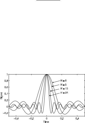
The Kaiser window is the same as the rectangular window when a equals 0. o½n& for N ¼ 20 and a ¼ 2, 4, 8, and 20 are shown in Figure 14.2. Increase of a at constant N reduces the sidelobes, but also increases the main lobe width. Increase of N at constant a reduces the main lobe width without appreciable change of sidelobes.

EXAMPLE 14.1 Rerun example 5.8 with apodization using the Hanning window along the x-direction. Compare the results along the x-direction and the y-direction. Solution: The Fraunhofer result obtained when apodization with the Hanning window along the x-direction is used with the same square aperture as shown in Figure 14.3. It is observed that there are less intense secondary maxima along the

TWO-POINT RESOLUTION AND RECOVERY OF SIGNALS

217

Figure 14.2. Kaiser windows for N ¼ 20, and a ¼ 2, 4, 8, and 20.

Figure 14.3. The intensity diffraction pattern from a square aperture in the Fraunhofer region when apodization with the Hanning window is used along the x-direction.

x-direction than along the y-direction. This is a consequence of the apodization along the x-direction.

14.3TWO-POINT RESOLUTION AND RECOVERY OF SIGNALS

Consider the Fraunhofer diffraction pattern from a circular aperture of radius R. As discussed in Example 5.8, the intensity distribution due to a plane wave incident on