Ufimtsev P. Fundamentals of the physical theory of diffraction (Wiley 2007)(348s) PEo

212 Chapter 7 Elementary Acoustic and Electromagnetic Edge Waves

7.16Find the vector-potential dA(x1,z) generated by the nonuniform current jx(1,z) induced on elementary strip 1 (Fig. 7.3). Follow the procedure shown below:

•Start with Equation (1.89). Substitute there the current jx(1,z) found in Problem 7.14.

•Use Equation (7.21) for the Green function.

•Calculate the integral over variable ξ1 (along the strip) in closed form.

•Apply the Cauchy theorem to the integral over variable η.

•Apply the asymptotic procedure (7.69) to integrals of the type of Equation (7.68).

•Represent the vector-potential in the form of a spherical wave diverging from the stationary point.

When you have this result, use Equations (1.92) and (1.93) and obtain the asymptotic expression for the wave generated by elementary strip 1. Having this, use the replacements

H0z → −H0z, β1 → β2, σ1 → σ2, ϕ0 → α − ϕ0, ϕ → α − ϕ,

and obtain the wave generated by strip 2. The sum of these waves is the EEW shown in Equation (7.130).

7.17Section 7.9.1 develops the asymptotics of acoustic EEWs free from the grazing sin-

gularity. Show that for the directions of the diffraction cone (ϑ = π − γ0), functions

Fh,s(1) take the form of Equations (7.167) and (7.168). Then prove Equations (7.173) and (7.174) for the specular direction ϕ = π − ϕ0 and verify Equations (7.177) and (7.178) for the grazing incidence (ϕ0 = π ) and the grazing scattering (ϕ = 0).

7.18Section 7.9.2 develops the asymptotics of electromagnetic EEWs free from the grazing singularity. Show that for the directions of the diffraction cone (ϑ = π − γ0), functions

F	G
(1),	(1) take the form of Equations (7.191) and (7.192). Then verify the relationships

(7.193) and (7.194) between acoustic and electromagnetic waves.

TEAM LinG

Chapter 8

Ray and Caustics Asymptotics for Edge Diffracted Waves

This chapter is based on the papers by Ufimtsev (1989, 1991).

8.1RAY ASYMPTOTICS

The following relationships exist between the acoustic and electromagnetic diffracted rays:

us = Et , if uinc(ζ ) = Etinc(ζ );	uh = Ht ,	if uinc(ζ ) = Htinc(ζ ),
where ˆt is the tangent to the edge at the diffraction point		ζ .

8.1.1 Acoustic Waves

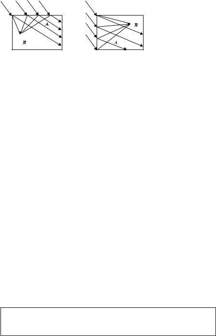
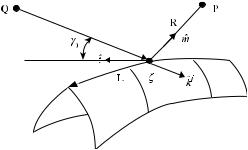
The theory of EEWs is applied here for calculation of scattering at a smoothly curved edge L with a slowly changing angle α(ζ ) between its faces (Fig. 8.1). In a small vicinity of the point ζ on the edge, an arbitrary incident field

uinc(ζ ) = u0(ζ )eikφ i (ζ )

(8.1)

can be locally considered as a plane wave propagating in the direction

ki	=	φi	=	grad	φi.	(8.2)
ˆ

Therefore, replacing the quantity uinc(ζ ) in Equations (7.89) and (7.90) and Equations (7.96) and (7.97) by Equation (8.1), we obtain the asymptotic expressions

Fundamentals of the Physical Theory of Diffraction. By Pyotr Ya. Ufimtsev

Copyright © 2007 John Wiley & Sons, Inc.

213

TEAM LinG

214 Chapter 8 Ray and Caustics Asymptotics for Edge Diffracted Waves

Figure 8.1 Element of a scattering edge L with a curvilinear coordinate ζ along the edge; ˆt is the unit vector tangential to the edge at the point ζ .

for EEWs generated by an arbitrary incident wave. The resulting diffracted wave arising at the edge L and created by the nonuniform/fringe sources js,h(1) is a linear superposition of EEWs (7.89), (7.90),

us,h(1) =	1	L u0(ζ )Fs,h(1)(ζ , mˆ )	eik (ζ )	dζ ,	(8.3)
	2π		R(ζ )

and the edge wave generated by the total scattering linear superposition of EEWs (7.96), (7.97)

sources js,h(t) = js,h(0) + js,h(1) is a

us,h(t) =	1		L u0(ζ )Fs,h(t)(ζ , mˆ )		eik (ζ )	dζ .	(8.4)
		2π			R(ζ )
Here,
	mˆ = R,			= φi + R,			(8.5)

and R is the distance between the edge point ζ and the observation point P(x, y, z). Notice that the differential operator in Equation (8.2) acts on coordinates of the edge point ζ , but the operator in Equation (8.5) acts on coordinates x, y, z of the observation point P.

A high-frequency approximation (with k 1) of the scattered field can be obtained by the stationary-phase technique (Copson, 1965; Murray, 1984), whose details have been already considered in Section 6.1.2. The stationary point ζst is determined by the equation

dζ

=

· ˆ

=

+

· ˆ =

ˆ

− ˆ

· ˆ =

d

t

(φi

R)

t

(ki

m)

t

0.

(8.6)

ks the unit vector m directed from the stationary point ζ

st

to the observation

Denote by ˆ

ˆ

point . Then Equation (8.6) can be rewritten as

ˆ

t

ˆ

· ˆ

= −

0

ks

· ˆ =

ki

cos γ .

(8.7)

t

TEAM LinG

	8.1 Ray Asymptotics 215
ks form a cone with its axis along the tangent t to the
Thus, the scattering directions ˆ	ˆ

edge at the stationary point. Such a cone is shown in Figure 4.4.

The function describes the distance between the points Q and P along the straight lines Qζ and ζ P (Fig. 8.1). Hence, Equation (8.6) indicates that this distance is extremal (minimal or maximal) when the point ζ is stationary. In other words, the location of the stationary point ζst on edge L satisfies the Fermat principle.

In accordance with the stationary-phase technique, the first term of the asymptotic expression for the field (8.3), (8.4) equals

(1)

1

uinc(ζ

(1)

, ks)

eikR ∞

k (ζst )

(ζ −ζst )

2

u

s,h

=

st

)F

s,h

(ζ

st

ei

2

dζ ,

(8.8)

2π

R

ˆ

−∞

where (ζst ) = d2 (ζst )/dζ 2, and R is the distance between the stationary point ζst and the observation point P. Due to the equality

∞

2

i

π

e±ix dx = √π e±

4 ,

−∞

Equation (8.8) can be written as

(1)

inc

(1)

ks)

eiπ/4

eikR

,

us,h

= u

(ζst )Fs,h

(ζst , ˆ

√

R

2π k (ζst )

where

'

= '

ei π2 ,

if (ζst ) < 0.

(ζst )

| (ζst )|

(8.9)

(8.10)

(8.11)

In terms of the local spherical coordinates R, ϑ , ϕ (introduced in Fig. 7.3), the

(1)

have the directions ϑ

=

π

−

γ

, 0

≤

ϕ

≤

2π . For these directions,

ks

0

unit vectors ˆ

functions F

s,h

ks) are determined by Equations (7.115) and (7.116). Hence

(ζst , ˆ

us(1) = uinc

(ζst ) f (1)

(ϕ, ϕ0, α)

eiπ/4

eikR

(8.12)

'

R

and

2π k (ζst )

uh(1) = uinc

(ζst )g(1)(ϕ, ϕ0, α)

eiπ/4

eikR

(8.13)

'

R

2π k (ζst )

in the directions 0 ≤ ϕ ≤ α, and

us(1) = −uinc

(ζst ) f (0)(ϕ, ϕ0, α)

√

eiπ/4

eikR

(8.14)

R

2π k (ζst )

TEAM LinG

216 Chapter 8

Ray and Caustics Asymptotics for Edge Diffracted Waves

and

uh(1) = −uinc(ζst )g(0)(ϕ, ϕ0, α)

√

eiπ/4

eikR

(8.15)

R

2π k (ζst )

in the directions α < ϕ < 2π , related to the region inside the tangential wedge.

(1)

(0)

The total diffracted field us,htot radiated by the total sources j s,htot = j s,h

+ j s,h

is described

by

Equations (8.12)

and

(8.13), where

one

should replace

f (1)(ϕ, ϕ0, α),

g(1)(ϕ, ϕ0, α) by functions

f (ϕ, ϕ0, α),

g(ϕ, ϕ0, α). In

the

region

α < ϕ < 2π (inside the tangential wedge),

the total

diffracted

field

u(1)

+

u(0)

asymptotically equals zero, because u

(1)

= −u

(0)

in accordance with Equations (8.14)

and (8.15).

The above asymptotics for edge diffracted waves can be presented in another form that reveals their ray structure. To do this, we utilize the following differential

operations:

=

d

=

t

(φinc

+

R)

=

t

ki

t

·

R

= −

cos γ

t

R, (8.16)

dζ

ˆ ·

ˆ · ˆ

+ ˆ

0

+ ˆ ·

d

dγ0

d

R

dt

sin γ

t

R

ˆ

,

(8.17)

= dζ

=

+

dζ

· dζ

[

0 dζ

· ˆ +

dζ

·

ˆ =

R

− ˆ ·

]

d R

t

1

1

(t

R)2

,

(8.18)

dˆt

vˆ

.

(8.19)

dζ

= a

Here vˆ is the unit vector of the principal normal to the edge L, and a is the radius of

curvature of the edge.

R

= −ˆ

ˆ ·

R

= −ˆ · ˆ

=

At the stationary point,

cos γ0

. Therefore,

ks and t

t ks

d R

t

sin2

γ0

,

(8.20)

R

dζ

· ˆ =

dt

ks

v

ˆ

R

ˆ

· ˆ

.

(8.21)

· dζ

= −

a

In view of relationships (8.16)–(8.19) and (8.20), (8.21),

1

(ζst ) =

R

1

+

ρ

sin2 γ0,

(8.22)

where

1

1

dγ

0

ks

v

ˆ

· ˆ

.

(8.23)

ρ = sin γ0

dζ

− a sin γ0

TEAM LinG

8.1 Ray Asymptotics 217

The quantity ρ is a caustic parameter; it determines the distance (R = −ρ) along the ray from the edge to the caustic.

Now the edge diffracted field can be written in the ray form

us,h(1) = uinc(ζst ) · (DF) · (DC) · eikR,								(8.24)
where
DF =		√		1				(8.25)
			R|1 + R/ρ|
is the rays’ divergence factor, and
			e±i π4			f (1)(ϕ, ϕ0, α)
DC =	sin γ0			√		g(1)(ϕ, ϕ0, α)		(8.26)
					2π k

can be interpreted as the diffraction coefficient. The quantities R and R + ρ are

the two principal radii of curvature of the diffracted phase front. The upper sign in e±iπ/4 is taken if (ζst ) > 0 and the lower one if (ζst ) < 0. The last multiplier in Equation (8.24), eikR, is the phase factor.

The divergence factor shows how the edge waves, being cylindrical-like waves in the vicinity of the edge (R |ρ|),

(DF)eikR ≈

eikR

√

,

(8.27)

R

transform into spherical waves,

(DF)eikR ≈ '

ikR

e

,

|ρ|

(8.28)

R

at a large distance from the edge (R

ρ).

The total edge diffracted fields can be also represented in ray form (with kR 1)

(t)

1

ei π4

f (ϕ, ϕ

0

, α)

us,h

= uinc(ζst )

√

sin γ0√

+g(ϕ, ϕ0, α), eikR.

(8.29)

R(1 + R/ρ)

2π k

We note that all variable parameters and coordinates in Equation (8.29) relate to the stationary point ζst .

Notice that the PTD ray asymptotics (8.14), (8.15) with the second derivative(ζ ) is much easier for the calculation than the GTD form (8.29), which involves complicated calculations of the caustic parameter ρ(ζ ).

TEAM LinG

218 Chapter 8 Ray and Caustics Asymptotics for Edge Diffracted Waves

8.1.2Electromagnetic Waves

According to Equations (7.130) and (7.131), the EEWs diverging from a scattering edge L create the combined wave

E

(1,t)

=

1

(1,t)(ζ )

eikR(ζ )

dζ

2π

L E

R(ζ )

and

H(1,t) =

1

L [ R(ζ )

× E(1,t)(ζ )]

eikR(ζ )

dζ ,

2π Z0

R(ζ )

with

(1,t)(ζ )

= [

E0t (ζ )F(1,t)(ζ )

+

Z0H0t (ζ )G(1,t)(ζ )

eikφi (ζ ).

E

]

(8.30)

(8.31)

(8.32)

	integrands contain the fast oscillating factor exp		ik (ζ )	, where
Here, the	i	[	]
(ζ ) = R(ζ ) + φ		(ζ ). Therefore, the application of the stationary-phase technique

to these integrals results in the following ray asymptotics:

Eϑ(1)

=

Z0Hϕ(1)

Einc(ζst )

f

(1)(ϕ, ϕ , α)

eiπ/4

eikR

t

f (ϕ, ϕ

,0α)

(t)

(t)

= −

sin γ0

R

Eϑ

=

Z0Hϕ

0

√2π k (ζst )

and

Eϕ(1)

= −

Z0Hϑ(1)

Z0Hinc(ζst )

(1)(ϕ, ϕ , α)

eiπ/4

eikR

t

gg(ϕ, ϕ ,0α)

.

(t)

(t)

=

sin γ0

Eϕ

= −

Z0Hϑ

0

√2π k (ζst ) R

They can also be written in the form of Equation (8.29):

(8.33)

(8.34)

Eϑ(1)

Z0Hϕ(1)

Einc(ζ

)

f (1)(ϕ, ϕ0, α)

eiπ/4

eikR

=

t

st

f (ϕ, ϕ0, α)

,

(8.35)

(t)

(t)

2

Eϑ

=

Z0Hϕ

γ0

√2π k √R(1 + R/ρ)

= − sin

and

Eϕ(1)

= −

Z0Hϑ(1)

Z0Hinc(ζst )

(1)(ϕ, ϕ , α)

eiπ/4

eikR

t

gg(ϕ, ϕ ,0α)

.

(8.36)

(t)

(t)

2

=

γ0

√2π k

Eϕ

= −

Z0Hϑ

sin

0

√R(1 + R/ρ)

TEAM LinG

8.1 Ray Asymptotics 219

Taking into account Equations (7.149) and (7.150), one can represent these approximations in terms of the field components tangential to the scattering edge:

E(1)

= Etinc(ζst )

(1)(ϕ, ϕ , α)

eiπ/4

eikR

Et(t)

f f (ϕ, ϕ0

,0α)

√

,

(8.37)

R

2π k (ζst )

t

H(1)

= Htinc(ζst )

(1)(ϕ, ϕ , α)

eiπ/4

eikR

Ht(t)

gg(ϕ, ϕ0,0α)

√

.

(8.38)

R

2π k (ζst )

t

8.1.3Comments on Ray Asymptotics

•A comparison of Equations (8.12), (8.13) and (8.37), (8.38) reveals the following relationships between acoustic and electromagnetic diffracted rays:

us = Et ,	if uinc(ζ ) = Etinc(ζ )	(8.39)
uh = Ht ,	if uinc(ζ ) = Htinc(ζ ),	(8.40)

where ζ is the diffraction point on a scattering edge. These relationships (together with Equations (7.149), (7.150)) allow one to completely determine the field of electromagnetic rays diffracted at a perfectly conducting object, if one knows the acoustic rays diffracted at soft and rigid objects of the same shape and size. Notice that these relationships were established earlier, in the paper by Ufimtsev (1995).

•The ray asymptotics (8.29), (8.35), (8.36) (for the field generated by the total scattering sources j(t) = j(0) + j(1)) were postulated in the Geometrical Theory of Diffraction (GTD) (Keller, 1962). Now it is seen that GTD can be interpreted as the ray asymptotic form of PTD for the total diffracted field. Notice that the ray asymptotics of Equation (8.29) type (but in the Kirchhoff approximation) were obtained first by Rubinowicz (1924). In the paper by Ufimtsev (1995), it is shown that the above ray asymptotics can be easily obtained by the direct extension of the Rubinowicz theory.

•In contrast to PTD, GTD is not applicable in the regions where the field does not have a ray structure and where the actual diffraction phenomena happen (GO boundaries, foci, caustics). Several ray-based techniques have been developed to overcome the deficiencies of GTD (Kouyoumjian and Pathak, 1974; James, 1980; Borovikov and Kinber, 1994). Among them, the most developed for practical applications is the Uniform Theory of Diffraction (Kouyoumjian and Pathak, 1974; McNamara et al. 1990).

TEAM LinG

220 Chapter 8 Ray and Caustics Asymptotics for Edge Diffracted Waves

Figure 8.2 Rectangular facet of the scattering edge. The edge diffracted rays (solid arrows) exist only in region A and satisfy the boundary conditions there. Individual elementary edge rays (dotted arrows) in region B do not satisfy the boundary conditions, but they asymptotically cancel each other there.

•	The ray asymptotics (8.29), as well as (8.35), and (8.36) for the fields E(t), H(t)
	are invariant with respect to the permutations ϑ ↔ γ0, ϕ ↔ ϕ0, and therefore
	they satisfy the reciprocity principle. We note that these expressions are valid
	of the diffraction cone (ϑ	=	π	−	γ		). Away from this
	only in the directionstot					0
	cone, the total field us,h is asympotically (with k	→ ∞) equal to zero, due to
	the absence of the stationary point on the edge. In this region, the individual
	elementary edge waves asymptotically cancel each other.
•	The asymptotic expressions (8.29) (and E(t), H(t) in Equations (8.35), (8.36)
	satisfy the boundary conditions on the planar faces of the edge. A situation with
	these conditions is illustrated in Figure 8.2.

•The ray asymptotics are not valid at caustics (R = 0 and R = −ρ), where they predict an infinitely large field intensity. The caustic R = 0 is located at the edge itself. The caustic R = −ρ can be real or imaginary.A real caustic occurs outside

ˆs

the scattering object in the positive direction of the vector k .An imaginary caus-

ˆs

tic is located in the direction contrary to k . In particular, imaginary caustics may be inside the scattering body. The value (ζst ) > 0 relates to the case when the edge diffracted ray has not yet reached a caustic, and the value (ζst ) < 0 corresponds to the ray that has already passed a caustic and acquired there the additional phase shift equal to −π/2 (according to Equation (8.11)).

•The theory of EEWs developed in Chapter 7 allows one to calculate the edge diffraction field in the vicinity of any caustics away from the scattering edge. An example of such a calculation is considered in the following section.

8.2CAUSTIC ASYMPTOTICS

Caustic asymptotics are presented here for both acoustic and electromagnetic waves.

These asymptotics have the same structure and differ only in coefficients.

TEAM LinG

8.2 Caustic Asymptotics 221

8.2.1 Acoustic Waves

Suppose that the edge diffracted rays form a smooth caustic C (Fig. 8.3). It is the envelope of diffracted rays, where a high-intensity field concentrates. According to Section 8.1 the diffracted field away from the caustic (and in front of the caustic) is the sum of two rays coming from the stationary points ζ1 and ζ2 on the scattering edge L:

	u = u0(ζ1)	√	eiπ/4		eik (ζ1)	+ u0(ζ2)	√	e−iπ/4		eik (ζ2)	,
				F(ζ1)					F(ζ2)
					R1					R2
			2π k (ζ1)					2π k| (ζ2)|

(8.41)

where (ζ ) = φi(ζ ) + R(ζ ) and φi(ζ ) is the phase of the incident wave at the point ζ on the scattering edge. Depending on the type of the function F(ζ1,2), Equation (8.41) represents either the field us,h(1) generated by the nonuniform/fringe sources js,h(1) or the

field us,htot generated by the total scattering sources js,h(t) = js,h(1) + js,h(0). Specifically, the functions

Fs(1)(ζ1,2) = f (1)(ϕ1,2, ϕ01,02, α1,2),	Fh(1)(ζ1,2) = g(1)(ϕ1,2, ϕ01,02, α1,2)
		(8.42)
relate to the field us,h(1), and the functions
Fs(t)(ζ1,2) = f (ϕ1,2, ϕ01,02, α1,2),	Fh(t)(ζ1,2) = g(ϕ1,2, ϕ01,02, α1,2)	(8.43)

correspond to the field us,h(t) . We note that functions f , g, f (1), g(1) are defined in Equations (2.62), (2.64), (4.14), (4.15), and (3.55) to (3.57). The function (ζ1,2)

can be represented in the form of Equation (8.22).

The first term in Equation (8.41) describes the ray that did not yet reach the caustic and the second term relates to the ray that has already touched the caustic.

Figure 8.3 Edge diffracted rays at the point P in the vicinity of caustic C.

TEAM LinG