Ufimtsev P. Fundamentals of the physical theory of diffraction (Wiley 2007)(348s) PEo

242 Chapter 9 Multiple Diffraction of Edge Waves

The amplitude u0 of the equivalent wave is determined by the equation

∂ueq

1 ∂ueq

= = =

∂uinc

1

∂uinc

=

1

∂uinc

=

= − r ∂ϕ

=

= RQ

= rq

(9.51)

∂n

z r 0, ϕ ϕ0

∂n

∂ϑQ

ϑQ

0

∂ϕq

ϕq

0

and equals

eikRQ

∂v0

=

u0 =

ikRQ sin γ0

∂ϑQ

ϑQ

0 .

(9.52)

It can be written in the form

u0 = w0eikφi ,

(9.53)

where φi = RQ and

1

∂v0

=

w0 =

ikRQ sin γ0

∂ϑQ

ϑQ

0 .

(9.54)

According to the idea introduced in Section 9.2, the waves diffracted at edge L are

found by the differentiation of Equations (8.3), (8.4) with the simultaneous replacement of uinc(ζ ) = u0(ζ ) exp[ikφi(ζ )] by the quantity (9.53). As a result, the edge

waves generated by the nonuniform/fringe scattering sources ( js,h(1)) are determined as

(1)

=

1

∂Fs(1)(ζ ) eik[R(ζ )+RQ(ζ )]

dζ

(9.55)

us

L w0(ζ )

2π

∂ϕ0

R

and

(1)

=

1

∂Fh(1)(ζ ) eik[R(ζ )+RQ(ζ )]

dζ ,

(9.56)

uh

L w0(ζ )

2π

∂ϕ0

R

and the edge waves radiated by the total scattering sources ( js,h(t) = js,h(1) + js,h(0)) are described by

(t)

=

1

∂Fs(t)(ζ ) eik[R(ζ )+RQ(ζ )]

dζ

(9.57)

us

L w0(ζ )

2π

∂ϕ0

R

and

(t)

=

1

∂Fh(t)(ζ ) eik[R(ζ )+RQ(ζ )]

dζ .

(9.58)

uh

L w0(ζ )

2π

∂ϕ0

R

Their ray asymptotics can be derived by the stationary-phase technique demonstrated in Section 8.1. However, we can obtain them much faster by the differentiation of

TEAM LinG

9.4 Slope Diffraction: General Case 243

the ray asymptotics (8.12), (8.13) and (8.29) with the simultaneous replacement of ui(ζst ) by (9.53):

us(1) uh(1)

us(t) uh(t)

∂f (1)(ϕ, ϕ

, α)

eik(R+RQ),

1

eiπ/4

0

w0(ζst )

∂ϕ0

(9.59)

∂ϕ0

=

√R(1 + R/ρ) sin γ0

∂g(1)(ϕ, ϕ0,

√2π k

α)

1

eiπ/4

∂f (ϕ, ϕ0, α)

e

w0(ζst )

∂ϕ0

ik(R

+

RQ)

,

(9.60)

(ϕ, ϕ , α)

∂g

=

√R(1 + R/ρ) sin γ0

√2π k

0

∂ϕ0

where the stationary point ζst is calculated according to Equation (8.7) and the caustic parameter ρ = ρ(ζst ) is defined in Equation (8.23).

In view of Equation (9.54), the fields arising due to the slope diffraction are less in magnitude by a small factor 1/kRQ compared to the ordinary diffracted fields (8.12), (8.13) and (8.29).

Notice that the integral representations (9.55), (9.56), (9.57), and (9.58) allow the calculation of the slope diffracted field in the vicinity of caustics and foci.

9.4.2Electromagnetic Waves

Let us define an incident electromagnetic wave as
Einc = E0i eikRQ ,	Hinc = H0i eikRQ ,	(9.61)
where
E0i = Z0[H0i	× RQ].	(9.62)

i

Suppose that in the direction to the scattering edge L, the quantities E0, H0 have zeros, but their first normal derivatives are not equal to zero:

E0

= 0, H0i = 0

on L

(9.63)

∂E0i

=

1 ∂E0i

∂H0i

=

1 ∂H0i

=0,

=0 on L.

(9.64)

∂n

RQ

∂ϑQ

∂n

RQ

∂ϑQ

As in the previous section, one approximates the actual incident wave (in the vicinity of the edge L) by the equivalent wave with components

Eteq = −ikrE0eqt	sin γ0 sin(ϕ − ϕ0)e−ikz cos γ0 e−ikr sin γ0 cos(ϕ−ϕ0),	(9.65)
Hteq = −ikrH0eqt	sin γ0 sin(ϕ − ϕ0)e−ikz cos γ0 e−ikr sin γ0 cos(ϕ−ϕ0),	(9.66)

which are the derivatives of the ordinary plane wave with respect to the incidence angle ϕ0. The amplitudes of the equivalent wave are found with the requirement that

TEAM LinG

244 Chapter 9 Multiple Diffraction of Edge Waves

the normal derivatives of this wave (on the scattering edge) are equal to those of the actual incident wave:

∂Eteq

∂Eteq

eq

∂E0i t

ikR

=

∂n

= − r∂ϕ

= ik sin γ0E0t

=

RQ∂ϑQ e

,

(9.67)

z

r 0, ϕ

ϕ

Q

eq

eq

= =

= 0

ϑQ 0

∂Ht

∂Ht

eq

∂H0i t

R

=

= − r∂ϕ

= ik sin γ0H0t

=

RQ∂ϑQ e Q

∂n

z

r

=

0, ϕ

ϕ

.

(9.68)

=

=

0

ϑQ

0

Hence

eq

1

ikR

∂E0i t

=

E0t

=

ikRQ sin γ0

e

Q

∂ϑQ

(9.69)

ϑQ 0

and

eq

1

ikR

∂H0i t

=

H0t

=

ikRQ sin γ0

e

Q

∂ϑQ

.

(9.70)

ϑQ

0

As in the previous section, the elementary edge waves diffracted at edge L are found by the differentiation of Equations (7.135) and (7.136), with respect to the angle ϕ0 and with the simultaneous replacement of E0t (ζ ), H0t (ζ ) by the quantities (9.69), (9.70):

dE

dH

Here,

(t)(ζ )	=	E0eqt	(ζ )	∂
E			∂ϕ0

(t)	=		dζ	(t)(ζ )eikRQ(ζ )	eikR(ζ )
						,
		2π E			R(ζ )

(t) = [ × (t)]

R dE /Z0.

	(t)(ζ , ϑ , ϕ) + Z0H0eqt (ζ )	∂
F			G(t)(ζ , ϑ , ϕ).
		∂ϕ0

The total edge wave created by all EEWs is determined by the integrals

E

(t)

=

1

(t)(ζ )

eik[R(ζ )+RQ(ζ )]

dζ

2π

L E

R(ζ )

and

H

(t)

=

1

[

R

(t)(ζ )

]

eik[R(ζ )+RQ(ζ )]

dζ .

2π Z0 L

× E

R(ζ )

(9.71)

(9.72)

(9.73)

(9.74)

(9.75)

TEAM LinG

Problems 245

The ray asymptotics of this wave are found by the stationary-phase technique:

(t)

(t)

eq

eiπ/4

∂g(ϕ, ϕ0

, α) eik(R+RQ)

Eϕ

= −Z0Hϑ

= Z0H0t

sin2

√

√

,

(9.76)

γ0

2π k

∂ϕ0

R(1 + R/ρ)

(t)

(t)

eq

eiπ/4

∂f (ϕ, ϕ0, α) eik(R+RQ)

Eϑ

= Z0Hϕ

= −E0t

sin2 γ0

√

√

,

(9.77)

2π k

∂ϕ0

R(1 + R/ρ)

where, for all functions of the variable ζ , one should take their values at the stationary point ζst . In view of Equations (7.149) and (7.150), these expressions can be written in terms of the components parallel to the tangent ˆt(ζst ),

eiπ/4

Et(t) = E0eqt sin γ0√2π k

eiπ/4

Ht(t) = H0eqt sin γ0√2π k

∂f (ϕ, ϕ0, α)			√		eik(R+RQ)
							,		(9.78)
	∂ϕ0				R(1 + R/ρ)
	∂g(ϕ, ϕ0, α)			√		eik(R+RQ)
								.	(9.79)
	∂ϕ0					R(1 + R/ρ)

Their comparison with Equation (9.60) leads to the equivalence relationships between the acoustic and electromagnetic diffracted rays arising due to the slope diffraction:

			∂				∂
us = Et ,	if				uinc(ζst ) =				Etinc(ζst ),	(9.80)
		∂n				∂n
			∂				∂
uh = Ht ,	if				uinc(ζst ) =				Htinc(ζst ),	(9.81)
			∂n				∂n

where ζst is the diffraction point on the scattering edge.

PROBLEMS

9.1Use the asymptotic expression (9.10) for the grazing diffraction of acoustic waves, apply the stationary-phase technique, and confirm the ray approximation (9.11).

9.2Use the asymptotic expressions (9.19), (9.20) for the grazing diffraction of electromagnetic waves, apply the stationary-phase technique, and confirm the ray approximations (9.23), (9.25). Compare Equation (9.25) with Equation (9.11) and establish the equivalence relationship between acoustic and electromagnetic diffracted rays.

9.3Use the asymptotic expressions (9.36), (9.37) for the slope diffraction of acoustic waves, apply the stationary-phase technique, and confirm the ray approximations (9.38), (9.39).

9.4Use the asymptotic expressions (9.43), (9.44) for the slope diffraction of electromagnetic waves, apply the stationary-phase technique, and confirm the ray approximations (9.45), (9.46) and (9.47). Compare Equation (9.47) with Equation (9.39), and establish the equivalence relationship between acoustic and electromagnetic diffracted rays.

TEAM LinG

TEAM LinG

Chapter 10

Diffraction Interaction of Neighboring Edges on

a Ruled Surface

The following relationships exist between acoustic and electromagnetic diffracted waves in the directions belonging to the diffraction cone:

	inc	inc				∂usinc(ζ )
uh = Ht ,	if uh	(ζ ) = Ht	(ζ ),	us = Et ,	if
						∂n

∂Einc(ζ )

=t .

∂n

Here, ˆt(nˆ ) is the tangent (normal) to the edge at the diffraction point ζ . These relationships, together with Equations (7.149) and (7.150), allow one to determine all components of the electromagnetic diffracted wave.

Consider a diffraction interaction of two edges with a common face. If this face is bent, the edge wave already undergoes diffraction on its way along the face to another edge. This problem is not amenable to theoretical treatment in a general case. However, the disturbing effect of the face can be neglected in the particular case illustrated in Figure 10.1. The common face S of edges L1 and L is a ruled surface whose generatrices coincide with the edge-diffracted rays arising at the edge L1 and propagating to the edge L. It is assumed that a plane tangential to the face does not change its orientation along the generatrix. Notice that a planar facet can be considered as a limiting case of a ruled surface. Therefore, the theory developed in the following is applicable in this case as well.

The present section is based on the papers by Ufimtsev (1989, 1991).

Fundamentals of the Physical Theory of Diffraction. By Pyotr Ya. Ufimtsev

Copyright © 2007 John Wiley & Sons, Inc.

247

TEAM LinG

248 Chapter 10 Diffraction Interaction of Neighboring Edges on a Ruled Surface

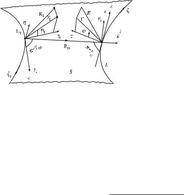
Figure 10.1 Element of a ruled surface S with two edges (L1 and L). The unit vectors ˆt1, ˆt are tangential to the edges. The unit vectors τˆ1, τˆ are tangential to the surface S and perpendicular to ˆt1, ˆt, respectively. The quantities r1, ϕ1, z1 and r, ϕ, z are local polar coordinates. The unit vector nˆ is normal to the plane tangential to S and containing the generatrix R10 as well as the tangents ˆt1, ˆt and τˆ1, τˆ. (Reprinted from Ufimtsev (1989) with the permission of the Journal of Acoustical Society of America.)

10.1 DIFFRACTION AT AN ACOUSTICALLY HARD SURFACE

Suppose that the edge wave propagating from the edge L1 has a ray structure and can be represented in the form of Equation (8.29) as

u1h(R1, ϕ1) = u01g(ϕ1, ϕ01, α1)		√	eikR1+iπ/4
	sin γ01			,	(10.1)
			2π kR1(1 + R1/ρ1)

where the function g(ϕ1, ϕ01, α1) is defined in Equation (2.64). In the vicinity of the edge L, this wave can be approximated by the two merging plane waves

lim

1

u

1h

(R

10

, 0)e−ikz cos γ0

(e−ikr sin γ0 cos(ϕ−ϕ0)

+

e−ikr sin γ0 cos(ϕ+ϕ0)). (10.2)

2

ϕ0

→

0

The first term here plays the role of the incident wave in the canonical wedge diffraction problem utilized in Chapter 7 to derive the asymptotic approximation (8.3), (8.4). Therefore, replacing the quantity u0(ζ ) exp(ikφi) in Equation (8.4) by (1/2)u1h(R10, 0), we obtain the asymptotic expression

uh(t) =	1	L u1h(ζ )Fh(t)(ζ , mˆ )	eikR(ζ )	dζ ,	with u1h(ζ ) = u1h(R10, 0), (10.3)
	4π		R(ζ )

for the edge wave generated by the total scattering source jh(t) = jh(1) + jh(0). One should note that in this particular case, jh(0) = u1h(R1, 0).

The ray asymptotic of this wave can be found by the stationary-phase technique. However, it can be obtained directly from Equation (8.29) if we replace there uinc(ζst ) by (1/2)u1h(ζst ) and set ϕ0 = 0:

TEAM LinG

10.1 Diffraction at an Acoustically Hard Surface 249

(t)	=	1				eikR+iπ/4
uh			u1h	(ζst )g(ϕ, 0, α)		√			,	(10.4)
		2
					sin γ0		2π kR(1	+ R/ρ)

where

u1h(ζst ) = u01g(0, ϕ01, α1)		√	eikR10+iπ/4
	sin γ01			.	(10.5)
			2π kR10(1 + R10/ρ1)

The letters α1, α denote the external angles of edges L1, L (π ≤ α1 ≤ 2π , π ≤ α ≤ 2π ), and the caustic parameters ρ1, ρ are defined according to Equation (8.23).

The ray asymptotic (10.4) is not applicable near the shadow boundary ϕ = π , where it becomes singular. Instead, one can suggest the following heuristic approximation of Equation (10.3) valid in all directions along the diffraction cone (ϑ = π − γ0, 0 ≤ ϕ ≤ α):

uh(t) = u1h			√	eikR
	(R10	, 0)Dh(χ , ϕ, γ0)				,	(10.6)
				R(1
					+ R/ρ)

where

Dh(χ , ϕ, γ0) =

χ

v(kχ sin γ0, ϕ)e−ikχ sin γ0 ,

(10.7)

sin γ0

2

sin

π

cos

ϕ

ϕ

N

e−iπ/4

sgn(cos 2 )∞ eit2 dt,

v(s, ϕ)

=

N

2

e−is cos ϕ

(10.8)

√

π

ϕ

π

√

cos

ϕ

2s

cos N

− cos N

2

with N = α/π , and

χ =

R10R

sin γ0.

(10.9)

R10 + R

According to the relationships

1

eis

v(s, π 0) =

(10.10)

2

and

ρ = ρ1 + R10,

for ϕ = π ,

(10.11)

TEAM LinG

250 Chapter 10 Diffraction Interaction of Neighboring Edges on a Ruled Surface

the diffracted field u(t) is discontinuous at the shadow boundary (ϕ1 = 0, ϕ = π ):

uh(t) =	1	+ R, 0).	(10.12)
	2 u1h(R10

However, the sum of the diffracted and incident fields (uh(t) + u1h) is continuous there. One can also show that the normal derivative of this sum is also continuous at the shadow boundary.

Utilizing the asymptotic approximation

[sgn(x)]∞	e	it2	dt −	eix2		with |x|
					,		1,	(10.13)
x				2ix

it is easy to verify

asymptotic		(10.4)			in
√2kχ sin γ0			ϕ2
		cos

that the uniform approximation (10.6) reduces to the ray the directions away from the shadow boundary, where 1.

10.2 DIFFRACTION AT AN ACOUSTICALLY SOFT SURFACE

The geometry of the problem is shown in Figure 10.1. Suppose that the edge wave

u1s(R1, ϕ1) = u01 f (ϕ1, ϕ01, α1)		√	eikR1+iπ/4	(10.14)
	sin γ01
			2π kR1(1 + R1/ρ1)

propagates from the edge L1 along the face S and, due to the boundary condition, equals zero in the direction ϕ1 = 0 to the edge L. We note that f (0, ϕ01, α1) = 0 in accordance with the definition given by Equation (2.62). Thus, the diffraction of the wave (10.14) at the edge L is a particular case of the slope diffraction, and it can be treated, as shown below, with a little modification of the technique developed in Chapter 9.

First, we notice that an appropriate wave (equivalent to the incident wave (10.14) in the vicinity of edge L) can be constructed from the combination of the incident and reflected plane waves

e−ikz cos γ0 (e−ikr sin γ0 cos(ϕ−ϕ0) − e−ikr sin γ0 cos(ϕ+ϕ0))

(10.15)

running along the face to the edge. Namely,

useq = u0eq e−ikz cos γ0

∂

(e−ikr sin γ0 cos(ϕ−ϕ0) − e−ikr sin γ0 cos(ϕ+ϕ0))|ϕ0=0

∂ϕ0

= −u0eq2ikr sin γ0 sin ϕ e−ikz cos γ0 e−ikr sin γ0 cos ϕ .

(10.16)

The amplitude factor ueq

of the equivalent wave is determined by the requirement

0

1

∂u1s

(R1, ϕ1)

1

∂useq

R10 sin γ01

∂ϕ1

R1

R10, ϕ1

0

=

r

∂ϕ

z r 0, ϕ

0

(10.17)

=

=

=

= =

TEAM LinG

10.2 Diffraction at an Acoustically Soft Surface 251

and equals

eq	1			∂u1s(R1, ϕ1)		=		=
u0	= −	i2kR10 sin γ01 sin γ0		∂ϕ1	R1		R10, ϕ1		0 .	(10.18)

According to the idea introduced in Chapter 9, the edge wave arising due to the slope diffraction of the equivalent wave (10.16) is determined by the derivative of (8.4) with the simultaneous replacement of u0(ζ ) exp(ikφi) by u0eq:

	1			∂		=			eikR(ζ )
us(t) =	2π	L u0eq	(ζ ) ∂ϕ0		Fs(t)(ζ , mˆ ) ϕ0		0	·	R(ζ )	dζ .	(10.19)

The ray asymptotic of the diffracted field (10.19) can be found by the stationary-

phase technique or directly by the differentiation of Equation (8.29) with the replacement of u0(ζ ) exp(ikφi) by u0eq:

(t)	eq		∂f (ϕ, 0, α)		eikR+iπ/4
us	= u0	(ζst )		sin γ0	√		.	(10.20)
			∂ϕ0			2π kR(1 + R/ρ)

This function is singular in the direction of the shadow boundary (ϕ = π ). Instead of it one can suggest the following heuristic approximation of Equation (10.19) valid in all directions along the diffraction cone (ϑ = π − γ0, 0 ≤ ϕ ≤ α):

	(t)	=	i ∂u1s(ζst )					eikR
	us					Ds(χ , ϕ, γ0)	√		,	(10.21)
			k		∂n
								R(1 + R/ρ)

where

∂u1s(ζst )

1

∂u

(R1, ϕ1)

=

=

∂n

=

R10 sin γ01

1s∂ϕ1

R1

R10,ϕ1 0

,

Ds(χ , ϕ, α) = −kχ

χ

ikχ sin γ0

w(kχ sin γ0, ϕ)e−

,

sin γ0

and

χ =

R10R

sin γ0.

R10 + R

Here,

2√

π

ϕ

ϕ

sin

sin

cos2

&

ei(s−π/4)

2

ϕ

N

N

2

w(s, ϕ) = −

%cos

π

ϕ

&2 F %√

2s

cos

√

,

N2

2

− cos

π s

N

N

(10.22)

(10.23)

(10.24)

(10.25)

TEAM LinG