Ufimtsev P. Fundamentals of the physical theory of diffraction (Wiley 2007)(348s) PEo

82 Chapter 4 Radiation by the Nonuniform Component of Surface Sources

incident at a perfectly conducting wedge, the following aymptotics diffracted far field (Ufimtsev, 2003):

(0)

= [E0z f

(0)

(ϕ, ϕ0) − H0z cos γ ]

eik1r+iπ/4

ikz cos γ

Ez

√

e

,

2π k1r

(0)

= H0zg

(0)

eik1r+iπ/4

ikz cos γ

Hz

(ϕ, ϕ0)

√

e

,

2π k1r

describe the

(4.54)

(4.55)

(1)

= [E0z f

(1)

(ϕ, ϕ0, α) + H0z cos γ ]

eik1r+iπ/4

ikz cos γ

Ez

√

e

,

(4.56)

2π k1r

(1)

= H0zg

(1)

eik1r+iπ/4

ikz cos γ

Hz

(ϕ, ϕ0, α)

√

e

.

(4.57)

2π k1r

The second term inside the brackets in Equation (4.54) shows the polarization coupling in the PO field under the oblique incidence. It also reveals itself in the second term of Equation (4.56). However, the field generated by the total surface current

(t) = (0) + (1)

j j j is free from this polarization coupling,

(t)		eik1r+iπ/4					ikz cos γ
Ez	= E0z f (ϕ, ϕ0, α)	√				e		,	(4.58)
				2π k1r
(t)	= H0zg(ϕ, ϕ0, α)	eik1r+iπ/4					ikz cos γ
Hz		√				e		.	(4.59)
			2π k1r

One should mention that the diffraction cone was first discovered theoretically for arbitrary curved edges by Rubinowicz (1924). In the case of curved edges, the axis of the diffraction cone is directed along the tangent to the edge at the diffraction point. He made this discovery by the asymptotic evaluation of the Kirchhoff diffraction integral (Rubinowicz, 1924). He also established that the edge diffracted rays satisfy Fermat’s principle. Later on, this concept of edge diffracted rays was included into the Geometrical Theory of Diffraction (Keller, 1962). The ray interpretation of the edge diffracted waves (4.48) and (4.49) was also suggested in the PTD (Ufimtsev, 1962). Senior and Uslenghi (1972) proved the existence of these rays in experiments with the diffraction of laser radiation.

PROBLEMS

Functions f (ϕ, ϕ0, α), g(ϕ, ϕ0, α) as well as functions f (0)(ϕ, ϕ0), g(0)(ϕ, ϕ0) are singular at the geometrical optics boundaries of the incident and reflected rays. Verify that their differences

f(1)(ϕ, ϕ0, α) and g(1)(ϕ, ϕ0, α) are finite there.

4.1Prove Equation (4.16).

4.2Prove Equation (4.17).

4.3Prove Equation (4.18).

4.4Prove Equation (4.19).

TEAM LinG

Chapter 5

First-Order Diffraction at

Strips and Polygonal

Cylinders

The relationship us = Ez and uh = Hz exist between the acoustic and electromagnetic

fields for these problems.

In Chapters 3 and 4, we have built a foundation for the solution of 2-D diffraction problems. General asymptotic expressions have been derived for the first-order edge diffracted waves generated both by the uniform and nonuniform components of the surface sources. In the present chapter, this general theory is applied to highfrequency diffraction at strips and cylinders with triangular cross-sections. These specific diffraction problems have been comprehensively studied in the existing literature. In particular, the uniform asymptotic expressions (with arbitrary high asymptotic precision) for the directivity pattern and for the surface field at the strips have been derived in Ufimtsev (1969, 1970, 2003). In these publications one can also find many other references related to the strip diffraction problem. Among them one should note the first and classical solution by Schwarzschild (1902). High-frequency diffraction at polygonal cylinders was investigated in Morse (1964) and Borovikov (1966). We now consider these problems again, to demonstrate the first applications of PTD.

5.1DIFFRACTION AT A STRIP

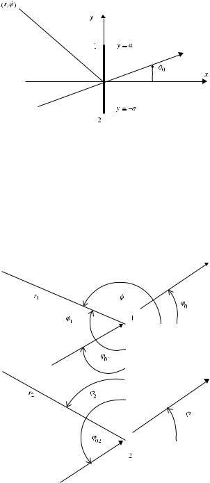
The geometry of the problem is shown in Figure 5.1. The soft (1.5) or hard (1.6) boundary conditions are imposed at the strip. The incident wave is given by

uinc = u0eik(x cos φ0+y sin φ0),

with − π/2 < φ0 < π/2.

(5.1)

Fundamentals of the Physical Theory of Diffraction. By Pyotr Ya. Ufimtsev

Copyright © 2007 John Wiley & Sons, Inc.

83

TEAM LinG

84 Chapter 5 First-Order Diffraction at Strips and Polygonal Cylinders

Figure 5.1 Cross-section of the strip by the plane z = const.

The diffracted field is investigated around the strip in the directions −π/2 <				φ < 3π/2.
For description of edge waves we utilize the local coordinates r1				, ϕ1, ϕ01
and r2, ϕ2, ϕ02, which are measured from the illuminated side of				the strip
(Fig. 5.2).

Figure 5.2 Local coordinates for edge waves.

TEAM LinG

5.1 Diffraction at a Strip

85

5.1.1Physical Optics Part of the Scattered Field

The Physical Optics (PO) part of the scattered field generated by the uniform components (1.31) of the surface sources is determined by the integrals (1.32). However, this integration process can be avoided. It turns out that the far field can be immediately calculated as the sum of two edge waves described in general form by Equations (3.53) and (3.54):

(0)

= u0

f

(0)

ei(kr1+π/4)

+ f

(0)

ei(kr2+π/4)

,

us

(ϕ1, ϕ01)

√

(ϕ2, ϕ02)

√

(5.2)

2π kr1

2π kr2

(0)

ei(kr1+π/4)

ei(kr2+π/4)

uh

= u0

g(0)(ϕ1, ϕ01)

√

+ g(0)(ϕ2, ϕ02)

√

.

(5.3)

2π kr1

2π kr2

For the far zone (r

)

us(0) = u0 f (0)

)

uh(0) = u0 g(0)

where

ka2), these expressions can be simplified:

(1)eika(sin φ0	−sin φ) + f (0)(2)e−ika(sin φ0−sin φ)*	ei(kr+π/4)
		√						,	(5.4)
			2π kr
	−sin φ) + g(0)(2)e−ika(sin φ0−sin φ)*	i(kr			π/4)
(1)eika(sin φ0		e√		+				,	(5.5)

2π kr

f (0)(1) ≡ f (0)(ϕ1	, ϕ01),	f (0)(2) ≡ f (0)(ϕ2, ϕ02),	(5.6)
and
g(0)(1) ≡ g(0)(ϕ1	, ϕ01),	g(0)(2) ≡ g(0)(ϕ2, ϕ02).	(5.7)

In accordance with Equation (3.55), functions f (0) and g(0) are defined in terms of the basic coordinates φ and φ0 as

f (0)(1) = −f (0)(2) =		cos φ0			(5.8)
		sin φ0 − sin φ
and
g(0)(1) = −g(0)(2) =		cos φ
			,		(5.9)
	sin φ0 − sin φ

with −π/2 < φ < 3π/2 and −π/2 < φ0 < π/2.

The field expressions (5.4) and (5.5) possesses a wonderful property. Although all functions (5.8) and (5.9) are singular for the directions φ = φ0 and φ = π − φ0,

their combinations in Equations (5.4) and (5.5) are always finite due to the relationships f (0)(1) = −f (0)(2) and g(0)(1) = −g(0)(2). This property of expressions

TEAM LinG

86 Chapter 5 First-Order Diffraction at Strips and Polygonal Cylinders

(5.4) and (5.5) becomes obvious when they are written in the explicit form

	(0)						(0)					ei(kr+π/4)
	us				= u0 s			(φ, φ0)				√			,			(5.10)
													2π kr
	(0)						(0)					ei(kr+π/4)
	uh				= u0 h			(φ, φ0)				√			,			(5.11)
													2π kr
where
(0)	(φ, φ	0		)		=	i2 cos φ		0		sin[ka(sin φ − sin φ0)]						,	(5.12)
s											sin φ − sin φ0
and
(0)(φ, φ			0		)	=	i2 cos φ			sin[ka(sin φ − sin φ0)]						.		(5.13)
h											sin φ − sin φ0
Now it is clear that
s(0)(φ0, φ0) = h(0)(φ0, φ0) = i2ka cos φ0																		(5.14)
for the forward direction φ = φ0, and
s(0)(π − φ0, φ0) = − h(0)(π − φ0, φ0) = i2ka cos φ0																		(5.15)

for the specular direction φ = π − φ0.

In accordance with the 2-D form of the optical theorem (Ufimtsev, 2003), the

total scattering cross-section is defined as
2
σ tot =		Im (φ0, φ0),	(5.16)
	k
which, following Equation (5.14), equals
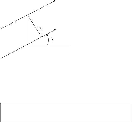
σs(0)tot = σh(0)tot = 2A,			(5.17)

where A = 2a cos φ0 is the “width” of the incident wave part intercepted by the strip (Fig. 5.3). Equation (5.17) can be also interpreted as the total scattered power per unit length of the strip in the z-axis direction.

It is expedient to introduce the 2-D bistatic scattering cross-section σ by a relationship similar to Equation (1.24):

Pavsc	=	σ · Pavinc	(5.18)
		2π r
			TEAM LinG

5.1 Diffraction at a Strip

87

Figure 5.3 Cross-section A of the incident wave intercepted by the strip.

where

	1			2			1			2
Pavinc =	2	k2Z u0			,	Pavsc =	2	k2Z usc	.		(5.19)

Therefore in view of Equations (5.10) and (5.11), the bistatic scattering cross-section is defined by

1				2
σs,h(0) =		s,h(0)	(φ, φ0) .		(5.20)
	k

This is a general definition of the bistatic scattering cross-section σ for any 2-D scattered fields represented in the form of Equations (5.10) and (5.11).

In the case of backscattering when φ = π + φ0, the directivity patterns are given by the simple expression

s(0) = − h(0) = i cot φ0 sin(2ka sin φ0).

(5.21)

Finally one should notice another peculiarity of the directivity patterns (5.12) and (5.13) for the field generated by the uniform components of the surface sources. They have exact zeros in the directions where

ka(sin φ0 − sin φ) = ±nπ ,	with n = 1, 2, 3, . . . .		(5.22)
This property is the consequence of the	relationships f (0)(1)	= −	f (0)(2) and
g(0)(1) = −g(0)(2).

5.1.2 Total Scattered Field

The nonuniform components of scattering sources concentrate near the edges of the strip and generate the two edge waves described by Equations (4.12) and (4.13). Their

TEAM LinG

88 Chapter 5

First-Order Diffraction at Strips and Polygonal Cylinders

sum equals

(1)

= u0

f

(1)

ei(kr1+π/4)

+ f

(1)

ei(kr2+π/4)

us

(ϕ1, ϕ01, 2π )

√

(ϕ2, ϕ02, 2π )

√

(5.23)

2π kr1

2π kr2

and

g(1)(ϕ1, ϕ01, 2π )

.

(1)

= u0

ei(kr1+π/4)

+ g(1)(ϕ2, ϕ02, 2π )

ei(kr2+π/4)

uh

√

√

(5.24)

2π kr1

2π kr2

As a result of relationships (4.12) and (4.13) and (4.14) and (4.15) these expressions can be written in the form

us(1) = us − us(0),

uh(1) = uh − uh(0).

(5.25)

Therefore, the total first-order scattered field is given by

(0)

(1)

= u0 f (ϕ1, ϕ01, 2π )

ei(kr1+π/4)

ei(kr2+π/4)

us = us

+ us

√

+ f (ϕ2, ϕ02, 2π )

√

2π kr1

2π kr2

(5.26)

and

= u0 g(ϕ1, ϕ01, 2π )

(0)

(1)

ei(kr1+π/4)

ei(kr2+π/4)

uh = uh

+ uh

√

+ g(ϕ2, ϕ02, 2π )

√

2π kr1

2π kr2

(5.27)

with functions f and g defined in Equations (2.62) and (2.64). For the far zone these field expressions are simplified to

us = u0 )f (1)eika(sin φ0−sin φ) + f (2)e−ika(sin φ0	−sin φ)*	ei(kr+π/4)
		√						(5.28)
				2π kr
and
uh = u0 )g(1)eika(sin φ0−sin φ) + g(2)e−ika(sin φ0	−sin φ)*	ei(kr+π/4)
		√					,	(5.29)
			2π kr

where
f (1) ≡ f (ϕ1, ϕ01, 2π ),	f (2) ≡ f (ϕ2, ϕ02, 2π ),
and	(5.30)
g(1) ≡ g(ϕ1, ϕ01, 2π ),	g(2) ≡ g(ϕ2, ϕ02, 2π ).

TEAM LinG

5.1 Diffraction at a Strip

89

In terms of basic coordinates φ and φ0, these functions are determined by

f (1)				1				1
g(1) =								2
				2			− sin		φ − φ0
and
f (2)	=	1						1
								2
g(2)		2				sin		φ − φ0

1 , with − π/2 ≤ φ ≤ 3π/2

cos

φ + φ0

2

(5.31)

2
1			, with π/2	φ	π/2, (5.32)
cos	φ + φ0		−	≤	≤

but

f (2)

1

1

1

,

with π/2 φ

3π/2.

2

2

≤

≤

φ − φ0

φ + φ0

g(2) =

2

− sin

± cos

(5.33)

As can be seen, functions g(2) and ∂f (2)/∂φ are discontinuous in the direction

φ= π/2. This is a consequence of the fact that they relate to the field generated by the scattering sources distributed over the whole half-plane −a < y < ∞. Functions g(1) and ∂f (1)/∂φ are also discontinuous. They have different values in the directions

φ= −π/2 and φ = 3π/2 related to the different sides of the half-plane −∞ < y < a containing the sources of the field.

This discontinuity in the field of the first-order edge waves (5.28) and (5.29) can be eliminated in two ways. First, in the calculation of the field generated by

the nonuniform component js,h(1), one should restrict the integration region by the actual surface of the strip. In other words, one should truncate (outside the strip) the component js,h(1) related to the semi-infinite half-plane. This approach is presented in Section 5.1.4 (see also Michaeli (1987) and Johansen (1996)). Another remedy is the calculation of multiple edge diffraction (Ufimtsev, 2003).

In view of Equations (5.31) to (5.33), the field expressions (5.28) and (5.29) can be written in the form

us,h = u0 s,h(φ, φ0)	ei(kr+π/4)
	√			,	(5.34)
		2π kr
					TEAM LinG

s(φ0, φ0) = i2ka cos φ0 −

(φ, ϕ0)) do not have

90 Chapter 5

First-Order Diffraction at Strips and Polygonal Cylinders

where

(φ, φ

)

= −

cos[ka(sin φ0 − sin φ)]

+

i

sin[ka(sin φ0 − sin φ)]

,

φ0 + φ

φ0 − φ

s

0

cos

sin

2

2

with

− π/2 ≤ φ ≤ π/2,

(5.35)

(φ, φ

)

=

cos[ka(sin φ0 − sin φ)]

−

i

sin[ka(sin φ0 − sin φ)]

,

φ0 − φ

φ0 + φ

s

0

sin

cos

2

2

with π/2 ≤ φ ≤ 3π/2,

(5.36)

and

(φ, φ

)

=

cos[ka(sin φ0 − sin φ)]

+

i

sin[ka(sin φ0 − sin φ)]

,

φ0 + φ

φ0 − φ

h

0

cos

sin

2

2

with

− π/2 ≤ φ ≤ π/2,

(5.37)

h

(φ, φ

0

)

=

cos[ka(sin φ0 − sin φ)]

+

i

sin[ka(sin φ0 − sin φ)]

,

φ0 − φ

φ0 + φ

sin

cos

2

2

with π/2 ≤ φ ≤ 3π/2.

(5.38)

As can be seen, these functions (in contrast to functions (s,h0) exact zeros in the directions determined by Equation (5.22).

In the following we provide the explicit expressions of functions s,h for certain specific directions of observation. For the forward direction φ = φ0,

1

(5.39)

cos φ0

and
1
h(φ0, φ0) = i2ka cos φ0 +					,			(5.40)
	cos φ0
and for the specular direction φ = π − φ0,
1
s(π − φ0, φ0) = i2ka cos φ0 −								(5.41)
		cos φ0
and
1
h(π − φ0, φ0) = −i2ka cos φ0 −							.	(5.42)
				cos φ0
In addition, for the backscattering direction φ = π + φ0,
		sin(2ka sin φ0)
s(π + φ0, φ0) = − cos(2ka sin φ0) + i								(5.43)
					sin φ0

TEAM LinG

5.1 Diffraction at a Strip

91

and

h(π + φ0, φ0) = − cos(2ka sin φ0) − i	sin(2ka sin φ0)	.	(5.44)
	sin φ0

In conformity with Equations (4.20) and (4.21), functions (5.39) to (5.42) are singular under the grazing incidence (φ0 = ±π/2).

A comparison with Equation (5.14) shows that the first term in Equations (5.39) and (5.40) is caused by the uniform component, and the second term by the nonuniform component of the surface sources. In view of Equation (5.16), this observation gives the impression that the field generated by the nonuniform component does not contribute to the total scattered power. An interesting question arises. How does it happen that the nonuniform component j(1) generates the field (5.23) and (5.24), but does not contribute to the total scattered power? The answer is the following. The field (5.23) and (5.24) does contribute to the total scattered field, but through the high-order edge waves generated due to multiple diffraction of the primary edge waves (5.34).

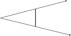
An additional comment is necessary on the field equations (5.28) and (5.29) and functions f and g involved in these equations. Functions f and g are singular in the forward (φ = φ0) and specular (φ = π − φ0) directions related to the geometrical optics boundaries of the incident and reflected rays. However, these singularities cancel each other in the field Equations (5.28) and (5.29) and provide finite values in these special directions, as is seen in Equations (5.39) to (5.42). This cancellation is due to the fact that the incident wave is a plane wave. Because of this, the geometrical optics boundaries related to the different edges of the strip are parallel to each other (Fig. 5.3) and merge in the far zone from the strip. This case represents an exception as compared to a more general situation when the source of the incident wave can be at a finite distance from the scattering object. For example, in the case of the cylindrical incident wave (Fig. 5.4), the shadow boundaries caused by the strip edges are not parallel and therefore the related singularities of functions f and g are separated in space and cannot cancel each other. In such a case, the traditional PTD procedure consists of the calculation of the fields generated separately by the uniform and nonuniform

Figure 5.4 Shadow boundaries caused by the strip edges in the field of the incident cylindrical wave. At these boundaries, functions f and g are singular: f = ∞ and g = ∞.

TEAM LinG