Ufimtsev P. Fundamentals of the physical theory of diffraction (Wiley 2007)(348s) PEo

132 Chapter 6 Axially Symmetric Scattering of Acoustic Waves at Bodies of Revolution

and

	1		0
g(1)(1) = g(1)(2) = ±		,	for ϑ = π	.	(6.80)
	2

After substitution of these values into Equations (6.41) and (6.42), it follows that

us(1)	= −	u0a eikR			,	for ϑ = 0 and ϑ = π ,		(6.81)
		2		R
and
(1)		u0a eikR				0
uh	= ±				,	for ϑ = π	.	(6.82)
		2		R

It is worth noting that the amplitude of the focal field generated by the nonuniform sources does not depend on frequency.

6.2.3 Total Scattered Field

The sum

us,h = us,h(0) + us,h(1)

(6.83)

provides the first-order PTD approximation for the scattered field:

•Quantities us,h(0) and us,h(1) are defined by Equations (6.56) and (6.57) and Equations (6.69) and (6.70).

•Their rays-type asymptotics are determined in Equations (6.60), (6.61) and (6.21), (6.22).

When they are included in Equation (6.83), the functions f (0), g(0) contained both in (6.60) and (6.61) and in (6.21) and (6.22) cancel each other. As a result, the ray asymptotics for the total field contain only the Sommerfeld functions f and g:

us =

√

u0a

)f (1)e−ika sin ϑ +i

π

+ f (2)eika sin ϑ −i

π

*

eikR

(6.84)

4

4

R

2π ka sin ϑ

and

uh =

√

u0a

)g(1)e−ika sin ϑ +i

π

+ g(2)eika sin ϑ −i

π

*

eikR

4

4

.

(6.85)

R

2π ka sin ϑ

Functions f (1, 2) and g(1, 2) are described by Equations (6.71) to (6.76), where the last terms (being outside the parentheses) should be omitted.

TEAM LinG

6.2 Scattering at a Disk 133

•The focal asymptotics for us,h(0) and us,h(1) are presented in Equations (6.58), (6.59) and, (6.81), (6.82). Their summation leads to

us = u0

ika2

1 +

i

eikR

,

for ϑ = 0 and

ϑ = π ,

(6.86)

2

ka

R

and

ika2

i

eikR

0

uh = ±u0

(1 −

)

,

for ϑ =

π

.

(6.87)

2

ka

R

Approximation (6.87) for the direction ϑ = π agrees with Equation (14.114) in the work by Bowman et al. (1987).

The results of numerical calculations shown in Figures 6.7 and 6.8 supplement the above analysis of the scattered field. The normalized scattering cross-section is the quantity

= σs,h σnorm π a2(ka)2

plotted in the decibel scale. The ordinary scattering cross-section σ is defined by Equation (1.26).

In Figures 6.7 and 6.8, the contribution to the scattered field generated by the nonuniform component of the scattering sources is clearly seen. The field scattered by the hard disk must be equal to zero in the direction ϑ = 90◦. The finite value of the PTD field in this direction (Fig. 6.8) is caused by the fictitious nonuniform sources distributed in the plane outside the disk surface. This shortcoming can be removed by the truncation of these fictitious sources, as was shown in Section 5.1.4.

Figure 6.7 Scattering at the acoustically soft disk. The curve “FRINGE” relates to the field generated by the nonuniform (“fringe”) scattering sources. According to Equations (1.100) and (1.101), the PO curve here also demonstrates the scattering of electromagnetic waves at a perfectly conducting disk.

TEAM LinG

134 Chapter 6 Axially Symmetric Scattering of Acoustic Waves at Bodies of Revolution

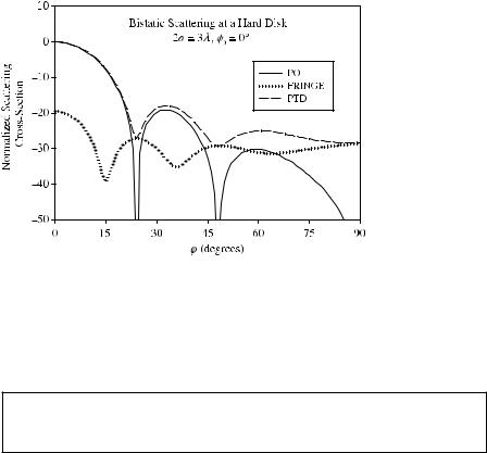
Figure 6.8 Scattering at the acoustically hard disk. The curve “FRINGE” relates to the field generated by the nonuniform (“fringe”) scattering sources. According to Equations (1.100) and (1.101), the PO curve here also demonstrates the scattering of electromagnetic waves at a perfectly conducting disk.

6.3SCATTERING AT CONES: FOCAL FIELD

The PO approximations for acoustic and electromagnetic focal fields in this problem are

identical. Asymptotics for the total acoustic and electromagnetic fields are different.

6.3.1 Asymptotic Approximations for the Field

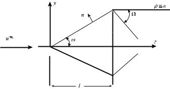
The geometry of the problem is shown in Figure 6.9. The incident plane wave is given by Equation (6.1). First, we calculate the focal field radiated by the uniform components js,h(0) of the induced scattering sources. They are defined by Equation (1.31) and determined on the cone surface by

js(0) = −2u0ik sin ωeikz

and

jh(0) = 2u0eikz.

(6.88)

The scattered field in the far zone is defined by Equations (1.16) and (1.17), where one should set

mˆ · nˆ = − sin ω cos ϑ ,	with ϑ = 0 or ϑ = π ,	(6.89)
and
ds = ξ sin ω dξ dϕ ,	with ξ = r .	(6.90)

TEAM LinG

6.3 Scattering at Cones: Focal Field 135

Figure 6.9 Cross-section of a cone by the plane yoz. A radius of the edge is a.

For the observation points on the focal line (ϑ = 0, π ), the integral over the variable ϕ equals 2π . Hence, the field us,h(0) can be represented in the form

				eikR				b
u(0)	=	u ik sin2		ω					eikξ(1−cos ϑ ) cos ωξ dξ		(6.91)
s		0			R			0
and
uh(0) = u0ik sin2			ω cos ϑ			eikR b				eikξ(1−cos ϑ ) cos ωξ dξ ,	(6.92)
							R		0

where b = a/ sin ω is the length of the cone generatrix and a is the radius of the edge. It follows from these equations that

us(0) = uh(0) = u0

ika2 eikR

(6.93)

2 R

in the forward direction (ϑ = 0), and

i

eikR

i

a

eikR

us(0) = −uh(0) = −u0

tan2 ω

+ u0

·

tan2 ω +

tan ω

ei2kl (6.94)

4k

R

4k

2

R

in the backscattering direction (ϑ = π ).

The forward scattering (6.93) is exactly the same as Equations (6.58) and (6.59) for the disk and actually represents the shadow radiation introduced earlier in Section 1.3.4. This result is in complete agreement with the Shadow Contour Theorem presented in Section 1.3.5, since the cone and the disk of radius a produce the same shadow and generate the same shadow radiation.

Comparison of the acoustic field, (6.93) and (6.94), with the electromagnetic PO field scattered by a perfectly conducting cone (Equation (2.4.3) in Ufimtsev (2003) reveals the relationships

TEAM LinG

136 Chapter 6 Axially Symmetric Scattering of Acoustic Waves at Bodies of Revolution

Ex(0) = us(0)	,	if Ex(0) = uinc	(6.95)
Hy(0) = uh(0)	,	if Hy(0) = uinc

for the directions ϑ = 0 and ϑ = π . This result is in complete agreement with the general relationships (1.100) and (1.101).

The field radiated by the nonuniform components of the scattering sources js,h(1) (induced near the circular edge on the cone) was investigated in Section 6.1. According to Equations (6.41) and (6.42), this field equals

(1)

= u0af

(1) eikR

us

R

and

(1)

= u0ag

(1) eikR

uh

R

in the forward direction ϑ = 0, and

(1)

= u0af

(1) eikR

e

i2kl

us

R

and

(1)

= u0ag

(1) eikR

e

i2kl

uh

R

in the backscattering direction ϑ = π . Here,

1

sin

π

1

π

1

f

(1)

= −

n

n

−

cot

+

cot ω

π

−

π

+

2ω

2n

n

2

cos

cos

n

n

and

1

sin

π

1

π

1

(1)

n

n

−

g

=

cot

−

cot ω

π

−

π

2ω

2n

n

2

cos

n

cos

+

n

for the forward direction ϑ = 0, and

sin

π

f (1)

n

1

π

1

2ω

1

tan ω

π

=

n

cos

− 1

− cos

− cos

−

2

n

n

n

(6.96)

(6.97)

(6.98)

(6.99)

(6.100)

(6.101)

(6.102)

TEAM LinG

6.3 Scattering at Cones: Focal Field 137

and

sin

π

1

1

1

g(1)

=

n

+

tan ω

(6.103)

π

π

2ω

2

n

cos

n

− 1

+ cos n

− cos

n

for the backscattering direction ϑ = π . In these equations, n = 1 + (ω + )/π .

In contrast to the above noted equivalence of the PO acoustic and electromagnetic fields, the acoustic field us,h(1) generated by the nonuniform scattering sources is different from the electromagnetic field radiated by the nonuniform electric currents. The electromagnetic field is given by Equations (2.3.18) and (2.3.19) in Ufimtsev (2003) and is determined by a linear combination of functions f (1) and g(1), but in the acoustic case the field us(1) depends only on f (1) and the field uh(1) depends only on g(1).

The above equations describe the field us,h(1) generated only by the nonuniform scattering sources induced near the cone edge. There are two other types of nonuniform sources induced on the cone surface, which we have neglected here. The first is caused by the smooth bending of the surface, which is a small quantity inversely proportional to (kρ) at a distance far from the cone tip. Here ρ is a polar coordinate of the surface (ρ = a at the edge points). The second is the nonuniform component concentrated near the cone tip. It is caused by both the sharp tip and by the large curvature of the cone surface due to its smooth bending near the tip. At a far distance ξ from the tip, it is of the order 1/kξ . In the case of electromagnetic diffraction, it was shown (Ufimtsev, 2003) that in the backscattering direction (ϑ = π ) one can neglect the field radiated by these types of nonuniform scattering sources. The asymptotic analysis of the electromagnetic field scattered by a semi-infinite cone also confirms this observation (Felsen, 1955; Bowman et al., 1987).

Taking these comments into account, the first-order PTD approximation for the backscattered total field (at the focal line ϑ = π ) can be found by summation of

Equations (6.94), (6.98) and (6.99):

=

−

4ka

−

us

u0a

i

tan2 ω(1

ei2kl )

ei2kl

sin

π

ikR

1

1

e

n

(6.104)

π

π

ω

+

n

cos

n

− 1

− cos

− cos

2

R

n

n

and

uh

=

u0a

4ka

−

ei2kl )

i

tan2 ω(1

ei2kl

sin

π

eikR

1

1

n

.

(6.105)

π

π

2ω

+

n

cos

n

− 1

+ cos

− cos

R

n

n

TEAM LinG

138 Chapter 6 Axially Symmetric Scattering of Acoustic Waves at Bodies of Revolution

In the limiting case when ω → π/2 and the front part of the object (Fig. 6.9) transforms into the disk, the above equations for the backscattered field are reduced to

ika

1

sin

π

1

eikR

π

us

u0a

n

n

cot

(6.106)

π

=

2

+ cos

− 1

+

2n

n R

n

and

1

sin

π

eikR

ika

1

π

n

uh u0a

n

cot

(6.107)

π

=

−

2

+ cos

− 1

−

2n

n R

n

with n = (3/2) + ( /π ). Finally, with → π/2 these expressions transform into

ika2

a

eikR

us = u0

−

(6.108)

2

2

R

and

uh = −u0

ika2

+

a

eikR

,

(6.109)

2

2

R

which exactly coincide with Equations (6.86), (6.87) for the field scattered back from the disk.

6.3.2Numerical Analysis of Backscattering

For the field represented in the form

	eikR
us,h = u0 s,h				,	(6.110)
		R
the scattering cross-section is defined according to Equation (1.26) by
σs,h = 4π s,h 2 .					(6.111)
We calculated the normalized scattering cross-section
σs,hnorm =	σs,h				(6.112)
	π a2

in the decibel scale, that is, the quantity 10 log(σs,hnorm). Note that this normalized scattering cross-section is different from the one used in Section 6.2.3 for the disk problem.

According to Section 6.3.1, the PO predicts the following approximation

		i			2
σ (0) = σs(0) = σh(0) = π a2		2ka	tan2 ω(1 − ei2kl ) − tan ω ei2kl		.	(6.113)

TEAM LinG

						6.3 Scattering at Cones: Focal Field		139
In the limiting case when ω → π/2,
					σ (0) = π a2(ka)2.		(6.114)
Together with the contribution from the nonuniform scattering sources j(1)								, the
total backscattering cross-section equals							s,h
σs	=	π a2	i	tan2 ω(1	−	ei2kl )
			2ka

2

π

1

n

1

n

n −

−

sin

π

ei2kl

− n %

n &

1

− cos

π

2ω

and

cos

cos

π a2

σh

=

i

tan2 ω(1

−

ei2kl )

2ka

1

1

2

π

n

n

n −

−

sin

ei2kl

π

+ n %

n &

1

+ cos

π

2ω

cos

cos

with n = 1 + (ω + )/π .

In the limiting case when ω → π/2,

2

=

+

2

π

+ n

n

ika

sin

1

π

σs

π a2

n

n

cot

,

π

−

n

and

cos

1

2

2

=

−

+

π

− n

n

sin

1

π

n

σh

π a2

ika

n

cot

π

−

n

cos

1

2

2

(6.115)

(6.116)

(6.117)

(6.118)

with n = (3/2) + ( /π ).

Finally when both ω and are equal to π/2, and the cone transforms into the disk,

σs = π a2 |ika − 1|2	(6.119)
and
σh = π a2 |ika + 1|2 .	(6.120)

The normalized backscattering cross-section (6.112) of the cone was numerically analyzed as the function of three variables: the length l, the angle ω and the angle .

TEAM LinG

140 Chapter 6 Axially Symmetric Scattering of Acoustic Waves at Bodies of Revolution

Figure 6.10 Backscattering at a cone: dependence on the cone length l. According to Equation (6.95), the PO curve also represents the scattering of electromagnetic waves from a perfectly conducting cone.

The results are presented in the decibel scale as follows:

•For the calculation of Equation (6.112) as a function of the length l, the variables were set as

ω = 45◦, = 90◦, a = l tan ω = l, 10 ≤ kl < 30.

In this case, 1.5λ < l < 4.8λ and 3λ < 2a < 9.6λ. The results are demonstrated in Figure 6.10. As is seen here, the data for the hard cone are higher than those for the soft cone. The difference between them is about 15 dB. The PO data are approximately in the middle.

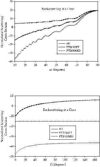
•For the calculation of Equation (6.112) as a function of the angle ω, the variables were set as

ka = 3π , 10◦ ≤ ω ≤ 90◦, = 90◦.

In this case, 2a = 3λ, 0 ≤ l ≤ 8.5λ. The results are plotted in Figure 6.11. A big difference can be observed between the soft and hard data here, at about 40 dB for narrow cones.

•For the calculation of Equation (6.112) as a function of the angle (Fig. 6.9), the variables were set as

ω = 10◦, ka = 3π , kl 17π , 0◦ ≤ ≤ π − ω = 170◦.

In this case, 2a = 3λ and l 8.5λ. The results are plotted in Figure 6.12. The PO approximation does not depend on the angle , which is why it is represented here by a straight horizontal line. The difference between the soft and hard data is about 42–57 dB. The influence of the cone base shape approaches 11 dB for the soft cone and 16 dB for the hard cone.

TEAM LinG

6.4 Backscattered Focal Fields 141

Figure 6.11 Backscattering at a cone: dependence on the vertex angle ω. According to Equation (6.95), the PO curve also represents the scattering of electromagnetic waves from a perfectly conducting cone.

Figure 6.12 Backscattering at a cone: dependence on the angle . According to Equation (6.95), the PO curve also represents the scattering of electromagnetic waves from a perfectly conducting cone.

6.4 BODIES OF REVOLUTION WITH NONZERO GAUSSIAN CURVATURE: BACKSCATTERED FOCAL FIELDS

This section studies symmetrical scattering at bodies of revolution whose illuminated side is an arbitrary smooth convex surface with nonzero Gaussian curvature. A generatrix of such a surface and related geometry are shown in Figure 6.13.

TEAM LinG