ivchenko_bookreg

2.1 Charge Carriers in Quantum Wells

31

By using the second equation of (2.45) one can express the vector spinor v via the gradient u as

P v =			2					u − i					2		[g(E) − g0](σ × )u ,					(2.47)
		2m(E)											4m0
where
1				2 P 2									2			1
			=													+		,		(2.48)
	m(E)			3			2					Eg + E					Eg + E + ∆
g(E) = g0 −						4 m0P 2											∆		.
						3				2				(Eg + E)(Eg + E + ∆)

Substituting (2.47) into the first equation of (2.45) we naturally come to a second-order di erential equation for the conduction-band envelope

2		ˆ2
		k
			u = E u .		(2.49)
	2m(E)
Therefore, in a bulk material the electron dispersion equation is
	2m(E)E = 2k2
or					(2.50)
E(E + Eg )(E + Eg + ∆) = P 2k2 E + Eg + 3 ∆ .
		2

Note that m−1(0) and the di erence g(0) −g0 describe the valence-band k ·p contributions to the inverse e ective mass and the g factor at the bottom of the conduction band (Sect. 5.3.3). Expanding the energy of the conduction band, Ec(k), to k4 we obtain from (2.50)

	2k2		η + η2		2k2
Ec(k) ≈		1 −	3 − 2			,	(2.51)
	2m		3 − η		2m Eg

where m = m(0) and η = ∆/(Eg + ∆). It should be mentioned that in (2.45) the term 2k2/(2m0) is dropped because it is comparable with the contribution of neglected remote bands. The generalized Kane model contains this dropped term as well as the quadratic-in-k term H(2). However, this modification deprives the model of its main asset, namely, the possibility of expressing all spectral parameters in terms of a limited number of the model constants.

The simplest boundary conditions for the envelope functions are the continuity of the spinor u(r) and of the normal component of the vector P v(r) at the interfaces. For a QW structure with the growth axis along z, they reduce to

uA = uB , PA (vz )A = PB (vz )B ,

(2.52)

32 2 Quantum Confinement in Low-Dimensional Systems

where PA, PB are values of P in materials A and B. One should bear in mind that if the energy E is referred to the conduction band bottom in the material A then, for the material B, the variable E in (2.45, 2.48, 2.49) must be replaced by E −EcB. The more general form of boundary conditions in the Kane model is analyzed in [2.37] (see also [2.38]).

For the states at kx,y = 0, spinor solutions of (2.48) can be presented in the form

us(z) = f (z) cs,

(2.53)

where f (z) is a scalar function and c1/2 = ↑, c−1/2 = ↓ are the spin-up and spin-down columns, respectively. In this case the boundary conditions take the form

fA = fB ,	1		df	A =	1		df		(2.54)
	mA(E)	dz			mB(E)	dz B

which di ers from the Bastard conditions (2.10) by using the energy-dependent (nonparabolic) e ective masses instead of those at the conduction band bottoms, mA and mB. Hence, the electron quantum-confinement energy at kx = ky = 0 satisfies the transcendental equations (2.12) and (2.14) where the fixed parameters mA, mB are replaced by the energy-dependent functions mA(E), mB(E).

2.2 Electron States in Quantum Wires and Nanotubes

In a QW, a free carrier can freely move in two directions. From this a QW structure is said to be a 2D system, or a quasi-2D system taking into account that the size-quantized states have a finite extension in the third direction as well. Now we turn to a brief overview of electron states in QWRs, or systems of the dimensionality d = 1, where the free motion is possible only in one direction.

2.2.1 Cylindrical and Rectangular Quantum Wires

In this subsection we consider the kind of QWRs in which one material, A, is surrounded by another material, B. In the e ective mass approximation, the 1D-electron envelope function is written in the factorized form

1
ψ(r) = √L eikz z ϕ(x, y) ,	(2.55)

where z if the QWR principal axis and L is its length. Sometimes, they use

the cylindrical coordinates, ρ = x2 + y2 and φ (the azimuth angle), rather than x, y. For QWRs, the boundary conditions (2.10) are changed to

ϕA = ϕB ,	1	(N · ϕ)A =	1	(N · ϕ)B	,	(2.56)
	mA		mB

2.2 Electron States in Quantum Wires and Nanotubes

33

where N is the normal to the dividing surface between materials A and B. In a cylindrical QWR, the electron states are characterized by a particular

z-component, M , of the angular momentum. For the axially-symmetric states with M = 0, the function ϕ(x, y) ≡ ϕ(ρ) is expressed via the Bessel functions J0(x) and K0(x) as follows

D K0(æρ) , if	ρ ≥ R ,
ϕ(x, y) = C J0(kρ) , if	ρ ≤ R ,	(2.57)

where R is the wire radius, k and æ are related with the energy E by the equations

k =	2	− kz2	1/2	, æ =	2		−		+ kz2	1/2
										(2.58)
	2mAE				2mB(V			E)

similar to (2.7). Taking into account (2.56) we have D = CJ0(kR)/K0(æR) and come to the following equation for the electron energy

J1(kR)K0(æR)	=	æ mA	.	(2.59)
J0(kR)K1(æR)
		k mB

In a QWR with an infinite confining potential, when the wave function at the boundary can be set to zero, this equations reduces to J0(kR) = 0. The first three zeros of the function J0(x) are 2.405, 5.520 and 8.654.

Let us now consider a less symmetrical QWR, namely, a QWR with the rectangular cross-section ax × ay along the axes x and y. In structures with infinitely high barriers, one has

ϕ(x, y) = ϕνx (x; ax)ϕνy (y; ay ) ,						(2.60)
where
ϕν (x; a) =		a		sin (νπx/a)	for even ν .	(2.61)
	2			cos (νπx/a)	for odd ν ,

Each electron subband is labelled by two quantum numbers νx, νy . The energy of an electron in the state (νx, νy , kz ) is given by

Eeνx νy kz	= 2mA	ax			+	ay		+ kz2	.	(2.62)
	2		νxπ	2			νy π	2

In the Kane model the electron states are described by the scalar and vector envelopes, u and v, satisfying equations (2.47, 2.49) and boundary conditions

uA = uB , PA (N · v)A = PB (N · v)B .

(2.63)

One can present the spinor wave function u(r) in the general form as

us(r) = [f (r) + i σαhα(r)] cs ,

(2.64)

34 2 Quantum Confinement in Low-Dimensional Systems

where cs (s = ±1/2) are the spin-up and spin-down states and, for kz = 0, f (r), hα(r) are real functions. Symmetry of a nanoheterosystem imposes restrictions on coordinate dependence of these functions. In particular, in

cylindrical wires, f (r) ≡ f ( x2 + y2) while the three functions hα(r) are identically equal to zero because there exist no polynomials l,m Cl,mxlym which transform as pseudovector components with respect to operations from the point group D∞h. Taking into account the nonparabolicity in the Kane model, the equation for the electron energy in the state with M = 0 is obtained from (2.59) by substituting mA(E), mB(E) instead of mA, mB.

For the conduction-electron state at the lowest-subband bottom kz = 0 in a rectangular QWR, the envelopes u, v are independent of z and, hence,

f (r) ≡ f (ρ) = f (x2, y2) , hz (ρ) = xyM (x2, y2) , hx(r) ≡ hy (r) ≡ 0. (2.65)

In the case of a quadratic cross section, one has

hz (ρ) = xy(x2 − y2)F (x2, y2) ,

(2.66)

where F (x2, y2) = F (y2, x2). The continuous envelopes f (ρ) and h(ρ) ≡ hz (ρ) satisfy equation (2.49), they are coupled at the interfaces by the continuity condition for the normal component of the spinor vector P v related to u by (2.47). This condition imposes the continuity requirement on the two following linear combinations of the derivatives f and h:

µ

Nx ∂x

+ Ny ∂y

− 2

Nx ∂y

− Ny ∂x

,

(2.67)

∂f

∂f

G

∂h

∂h

µ

Nx ∂x

+ Ny ∂y

+ 2

Nx ∂y

− Ny ∂x

,

∂h

∂h

G

∂f

∂f

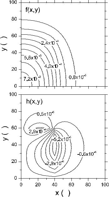
where Nx, Ny are components of the 2D unit vector N normal to the A/B boundary, and µ = m0/m(E) , G = g(E) − g0. In [2.39] the ground-state solutions |e11, s of (2.49) in a wire of the cross section 2a×2b were calculated using the free relaxation technique described in [2.40]. The envelopes f (ρ)

˚	˚
and h(ρ) calculated for the GaAs/Al0.35Ga0.65As QWR 80 A	× 120 A are

shown in Fig. 2.3 as contour maps. The origin of the coordinate system (x, y) is chosen in the wire center. Due to the rectangular symmetry, see (2.65), it is enough to present the variation of f and h only in the quadrant x, y > 0. The function f (x, y) has the maximum value fmax ≈ 7 × 10−3 at the center and monotonously decreases with increasing the radial distance ρ. In accordance with (2.65) the function h(x, y) is zero if x = 0 or y = 0. It follows from (2.66) that for coinciding a and b this function should vanish also at the diagonal x = y and have opposite signs at the points (x, y) and (y, x). One can see in Fig. 2.3 areas of opposite signs in the map of h(x, y) in spite of a remarkable di erence between a and b. As a result, in every quadrant the function h(x, y) exhibits a maximum and a minimum. As compared with fmax, the extremum values of h(x, y) are smaller by three orders of magnitude.

2.2 Electron States in Quantum Wires and Nanotubes

35

Å

Å

Å

Å
	Å
Fig. 2.3. Contour plots of the envelopes f (x, y) and h(x, y) for the electron lowest
subband e1 (at the bottom, kz = 0) in a 2a × 2b rectangular GaAs/AlGaAs QWR
˚	˚
with a = 40 A and b = 60 A. [2.39]

36 2 Quantum Confinement in Low-Dimensional Systems

In QWRs with a confining potential of complicated shape, e.g., in V- shaped QWRs, the electron and hole states are calculated by direct solution of the full 2D Schr¨odinger equation, see [2.41].

2.2.2 T-shaped Quantum Wires

We consider a T-shaped QWR consisting of a cleaved QW of the thickness a and an overgrown QW of the thickness b, see inset in Fig. 2.4a. As compared to the QWR structures discussed in the previous subsection, the confining potential in T-shaped wires has openings so that free carriers are classically unbounded in such structures. However, the quantum mechanics allows formation of bound electron or hole states at the T intersection. The binding energy, ε1D, of a 1D state is defined as an energy di erence Ee1(max{a, b}) − E1D between the lowest 2D-electronic state in the wider QW and the 1D-state under consideration. Here Ee1(a) is the e1-subband quantum-confinement energy in a single QW of the thickness a. The solid line in Fig. 2.4a shows the calculated dependence of the energy of the low-

˚

est wire-like electron state on the width b at fixed a = 50 A in the T-shaped GaAs/Al0.35Ga0.65As structure. Physically, it is clear that, with changing the width b, the electron wave function is redistributed between the cleaved and overgrown QWs. For b → 0, the energy E1D asymptotically approaches that of a 2D electron in the overgrown well (indicated in Fig. 2.4a by the dotted horizontal line). In the opposite case, with b increasing and becoming much larger than a, the electron penetrates more and more into the cleaved well and E1D → Ee1(b). The binding energy ε1D is represented in the figure by the dashed line. Note that ε1D is not an analytical function of b since at the point b = a the meaning of the lowest 2D state changes. It is this point at which the binding energy, or the 2D-1D separation, reaches a maximum. According to Kiselev and R¨ossler [2.42], this simple criterion, i.e., the equality of the minimum energy values of 2D states in cleaved and overgrown QWs, can be applied to much more complex structures fabricated by the cleaved edge overgrowth technique. The probability density of the lowest electron states

˚

in the QRW with a = b = 70 A is shown in Fig. 2.4b.

Some modifications of the conventional T-shaped structure can lead to an enhanced 2D-1D separation. One of the possibilities is the double T-shaped structure where two individual intersections are close enough to each other to permit ‘bonding’ and ‘antibonding’ 1D states. It is interesting to compare the tunnelling exponents that govern the coupling of 2D states in the cleaved QWs and of 1D states in the double T-shaped structure. According to (2.7), for the former coupling, it is exp (−æ2DLb) with Lb being the width of the barrier layer between two cleaved QWs and

æ2D = 2mB(V − Ee1)/ 2 .

The similar quantity exp (−æ2DLb) for the wire-like states is represented by

	2.2 Electron States in Quantum Wires and Nanotubes	37

Å

Å

Å

Fig. 2.4. (a) The dependence of the energy of the lowest electron state in a GaAs/Al0.35Ga0.65As T-shaped structure (shown in inset) on the width b of the

˚

cleaved QW (solid) for a fixed width of the overgrown QW, a = 50 A. The quantumconfinement energies of the lowest electron states e1 in the cleaved and overgrown QWs are represented by dotted lines. The 2D-1D di erence is shown as a dashed line. (b) The electon probability density for the wire-like electron state in the struc-

˚

ture with a = b = 70 A. From [2.42].

æ1D = 2mA(Ee1 − E1D)/ 2 .

Thus, there is a range of barrier widths Lb where coupling of well states is negligible and, at the same time, the interaction of the wire-like states is strong.

Langbein et al. [2.43] calculated and optimized the confinement energies for electrons and holes in T-shaped QWRs using the e ective-mass approximation for the simple conduction band and the six-band envelope-function theory (the Luttinger model) for the valence bands Γ8, Γ7. They showed that the conduction-band 1D state is confined more or less equally in di erent arms of the T-intersection, while the lowest valence-band state is more extended along the overgrown QW. This is a direct consequence of the isotropic conduction-band mass and the anisotropic valence-band mass. Moreover, due the large and anisotropic hole e ective mass, the 1D valence-band states are only weakly bound at the T-shaped intersection.

Calculations of bound states in other opened QWR structures can be found in [2.44] (H-shaped structure, or double QW connected by a bridge grown from the well material), [2.45, 2.46] (barrier-modulated wires), [2.47] (L-shaped QWRs).

38 2 Quantum Confinement in Low-Dimensional Systems

2.2.3 Carbon Nanotubes

We recall that a carbon nanotube is conceivable as a single hexagonal layer cut and rolled up into a cylinder. Thus, we start from the electron structure of a 2D graphite, or graphene. The carbon atoms in a graphene plane form a bipartite hexagonal lattice which can be divided into two sublattices A and

B.The 2D basis vectors with the angle 120◦ between them can be defined by

√

a = a(1, 0) , b = a		−	1	,	3	,	(2.68)
			2		2
where a is the lattice constant equal √		times the interatomic distance d =
	3

˚

1.44 A [2.48], and the coordinate system x, y in (2.68) is chosen in such a way that x a, y a and by > 0. The 2D reciprocal lattice is also hexagonal with the first Brillouin zone being a hexagon (Fig. 2.5).

Fig. 2.5. 2D Brillouin zone of graphene.

We choose one of the B sites as the origin (0,0) of the coordinate system.

Its three nearest A neighbors are located at the points
						1		√					−	1		√		. (2.69)
a		(0, −1) , r2	a						3		a						3
r1 = √			= √				,				, r3 = √				,
						2		2						2		2
	3			3								3

In the tight-binding theory, the electron wave function in the state with the wave vector k is written as

ψk(r) = Cα(k) exp [ik · (R + τα)]φ(r − R − τα) .	(2.70)

Rα

Here R is the 2D translational vector which enumerates the unit cells, α enumerates two carbon atoms in the unit cell belonging to the sublattices

2.2 Electron States in Quantum Wires and Nanotubes

39

A and B, τα is the position of the atom α within the unit cell and φ(r) is an atomic π orbital. The coe cients CA(k) and CB(k) written as a two-

ˆ

component column C(k) satisfy the following matrix equation

ˆ	ˆ
HC	= EC ,

where, in the nearest-neighbor approximation, the 2×2 e ective Hamiltonian is given by

	H =	E	h	3
				, h(k) = γ0 n=1 exp (ik · rn) ,	(2.71)
		h0	E0

γ0 is the nearest-neighbor transfer integral, E0 is the diagonal energy which in the following is set to zero. Substituting rn from (2.69) into the exponents one obtains [2.49, 2.50]

h = γ0	eiky a/√3 + 2e−iky a/2√3 cos 2 .						(2.72)
						kxa

The energy dispersion is given by E±(k) = ±|h(k)|. An important point is that the energy equals zero at each vortex of the 2D Brillouin zone (points K and K ), particularly at the left and right vortices

	K =	4π	(	1, 0) , K =	4π	(1, 0) .	(2.73)
		3a			3a
			−

Near these points the dispersion is linear, namely, E±(k ≈ K) = ±γ|k −K|. At zero temperature the states with negative energies are occupied (valence band) whereas those with positive energies are empty (conduction band). Thus, a graphene is a zero-gap 2D crystal in the sense that the conduction and valence bands consisting of π states touch at the K and K points.

Turning now to carbon nanotubes we write the circumferential vector as

L = naa + nbb ,

(2.74)

where na, nb are integers, and expand the electron e ective Hamiltonian for a graphene sheet in the vicinity of the points K and K [2.51, 2.52]. In the following we define k and k as wave vectors referred respectively to the points K and K and assume the products ka, k a 1 to be small. Then, in the second order in ka or k a, the nondiagonal matrix element (2.72) of the Hamiltonian H is given by (see [2.53, 2.54])

h(k, K) = γe−iθ k − ikz +

4√3 e3iθ (k + ikz )2

(2.75)

a

near the K point and

h(k , K ) = γeiθ −k

− ikz

+

a

e−3iθ (k − ikz )2

(2.76)

4√

3

40 2 Quantum Confinement in Low-Dimensional Systems

√

near the K point. Here γ = ( 3/2)γ0a, θ is the angle between the vector L and the basis vector a. The subscripts z, indicate components of a vector referred to the axes lying in the graphene plane and related to the vector L so as z L and kz L, k L. In the same approximation the energy spectrum near the K point is given by

Ec,v (k, K) = ±|h|			k3 − 3k kz2 cos 3θ +	kz3 − 3k2 kz		(2.77)
≈ ±γ |k| +	4√3 k					sin 3θ ,
	a
	| |

where |k| = k2 + kz2, the upper and lower signs represent the conduction (subscript c) and valence (subscript v) bands, respectively. The similar spectrum near the K point is obtained by changing k → −k , kz → kz , θ → −θ in agreement with the time inversion symmetry requirement Ec,v (k, K ) = Ec,v (−k, K).

In a carbon nanotube specified by the vector L the electron wave function satisfies the cyclic boundary condition Ψ (r) = Ψ (r + L). This enables one to find the allowed discrete values of k as

k =	2π	n −	ν	; k	=	2π	n +	ν	,	(2.78)
	L		3			L		3

where n is an integer 0, ±1, ±2... characterizing the angular momentum com-

ponent of an electron, L = |L| = a n2a + n2b − nanb, and ν equals one of three integers: 0, ±1 determined by the presentation of the sum na + nb as 3N + ν with integer N . In the e ective-mass approximation, the electron envelope functions can be written in the form

	einϕ		eikz z	ˆ
ψc,v (z; n, kz ) =	√		√LCN	Cc,v (n, kz ) ,	(2.79)
		2π

where LCN is the nanotube length and ϕ is the azimuth angle. The two-

ˆ
component columns Cc,v are eigenvectors of the 2×2 matrix Hamiltonian
(2.71), given by	√2				1| |	, Cˆv = √2	−h/|h|
Cˆc =			h					(2.80)
	1				/ h	1	1

with h defined by (2.75) for the 1D K-valley and by (2.76) for the 1D K - valley where K, K are the z-components of the vectors K, K .

The dispersion in the conduction and valence subbands is obtained by substituting (2.78) into (2.75, 2.76 or 2.77). In the linear approximation, the conduction and valence band spectra are given by

Ec,v (n, kz ; K) = ±γ		L	2	n − 3		+ kz2	,		(2.81)
		2π		ν		2
Ec,v (n, kz ; K ) = ±γ
		L	2	n + 3		+ kz 2 .
		2π		ν		2