

Коновалов Учебно-методическое пособие по курсу 2007
.pdfчисла узлов разбиения по координате, начиная с которых для заданного шага по времени проявляется нарушение сходимости численного решения задачи (21) к стационарному решению (22).
Таким образом, схема (25) устойчива при условии γ = ∆τ / ∆x2 <α ,
где α ≈ 0.75 .
На графиках после программы представлены примеры неустойчивости решения для некоторых значений временного шага ∆τ из рассмотренного диапазона (табл. 1) и γ > 0.75 .
Значения коэффициента ki достаточно определять по значениям si на предыдущем временном слое. Переопределение значений ki на каждом временном шаге по новым значениям si с
помощью итерационной процедуры, фактически, не влияет на конечный результат – расхождение в решениях (на конечный момент времени) без итераций и с десятью итерациями проявляется
в четвертом знаке после запятой для ∆τ =10−2 . Причиной является относительно малое значение шага по времени, начиная с которого схема (25) дает устойчивое решение.
|
Таблица 1. Значения шагов программы |
|
|
|
||||||||||||
|
|
∆τ |
2 10−2 |
10−2 |
5 10−3 |
|
2 10−3 |
10−3 |
5 10−4 |
2 10−4 |
||||||
|
|
|
Nmax |
8 |
|
10 |
14 |
|
21 |
29 |
40 |
63 |
||||
|
|
|
∆τ |
0.98 |
|
0.81 |
0.85 |
|
0.8 |
0.78 |
0.76 |
0.77 |
||||
|
|
|
∆x2 |
|
|
|
|
|
|
|
|
|
|
|
|
|
|
Продолжение табл. 1. |
|
|
|
|
|
|
|
|
|||||||
|
∆τ |
10−4 |
|
5 10−5 |
|
2 10−5 |
|
|
|
|
|
|||||
|
|
Nmax |
88 |
|
124 |
|
195 |
|
|
|
|
|
|
|||
|
|
∆τ |
0.76 |
|
0.76 |
|
0.75 |
|
|
|
|
|
|
|||
|
|
∆x2 |
|
|
|
|
|
|
|
|
|
|
|
|
||
21
>#============================================
>#======= 1D Ice Sheet Model (1D-model) ============
>#============================================
>restart:
>
>with(LinearAlgebra):
>#--------------------
>N_Glen:=3;
N_Glen:=3
> a:=0.3;
a :=0.3
> dens:=910;
dens:=910
> g:=9.8;
g :=9.8
> Ao:=1e-16;
Ao := 0.1 10 -15
> Lo:=10^5;
Lo:=10000
>
Zo:=(a*(N_Glen+2)*Lo^(N_Glen+1)/(2*Ao*(dens*g)^N_Glen))^(1/(
2*(N_Glen+1)));
Zo := 1007.006694
> To:=Zo/a;
To := 3356.688980
>#------------------------------------------------------------------------
>#-------- Steady State Ice Sheet, Analytic Solution -----------
>#------------------------------------------------------------------------
>
> Sa:=2^(N_Glen/(2*N_Glen+2))*(1- x^((N_Glen+1)/N_Glen))^(N_Glen/(2*N_Glen+2));
(3/8) |
(1 −x |
(4/3) |
(3/8) |
Sa :=2 |
|
) |
22
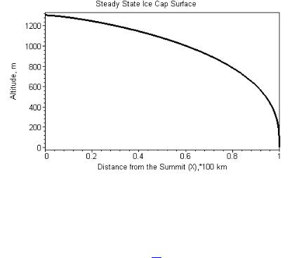
> plot(Zo*Sa,x=0..1,numpoints=10,axes=boxed,title="Steady State
Ice Cap Surface", labels=["Distance from the Summit (X),*100 km","Altitude, m"], labeldirections=[HORIZONTAL,VERTICAL], color=black,thickness=3);
>#--------------------------------------------------------------
>Nt:=2000;
Nt := 2000
> Nx:=21;
Nx:=21
> dx:=1/(Nx-1);
1 dx :=20
> dt:=0.001;
dt := 0.001
>#--------------------------------------------------------------
>N1:=100: N2:=200: N3:=300: N4:=500: N5:=800: N6:=1000:
>#--------------------------------------------------------------
>K_eff:=array(1..Nx-1):
>#------------------
>S:=array(1..Nx):
>So:=array(1..Nx):
>#--------------------------------------------------------------
>H_Ice_Summit:=array(0..Nt):
23
>#--------------------------------------------------------------
>M:=Matrix(Nx);
|
21 x 21 Matrix |
|
|
|
|
|
Data Type: anything |
|
M := |
|
|
|
Storage: rectangular |
|
|
|
|
|
Order: Fortran_order |
|
> V:=Vector(Nx); |
21 Element Column Vector |
|
|
||
|
Data Type: anything |
|
|
|
|
V := |
Storage: rectangular |
|
|
|
|
|
Order: Fortran_order |
|
|
|
|
>#-------------------------------------------------------------
>for i from 1 to Nx do S[i]:=0: end do:
>#-------------------------------------------------------------
>H_Ice_Summit[0]:=S[1]:
>#-------------------------------------------------------------
>for i from 1 to Nx do So[i]:=S[i]: end do:
>#-------------------------------------------------------------
>
> for m from 1 to Nt do
for Iitr from 1 to 1 do
for i from 1 to Nx-1 do K_eff[i]:=abs((So[i+1]-So[i])/dx)^(N_Glen- 1)*((So[i]+So[i+1])/2)^(N_Glen+2):
end do:
LL:=[[seq(-K_eff[i-1]/dx^2,i=2..Nx-1),0], [2*K_eff[1]/dx^2+1/dt,seq((K_eff[i-1]+K_eff[i])/dx^2+1/dt,i=2..Nx- 1),1],
[-2*K_eff[1]/dx^2,seq(-K_eff[i]/dx^2,i=2..Nx-1)]]:
M:=BandMatrix(LL):
for i from 1 to Nx-1 do V[i]:=1+S[i]/dt: end do:
S_solve:=LinearSolve(M,V):
24
for i from 1 to Nx do So[i]:=S_solve[i]: end do: end do:
for i from 1 to Nx do S[i]:=So[i]: end do:
if m=N1 then for i from 1 to Nx do S1[i]:=S[i]: end do: end if: if m=N2 then for i from 1 to Nx do S2[i]:=S[i]: end do: end if: if m=N3 then for i from 1 to Nx do S3[i]:=S[i]: end do: end if: if m=N4 then for i from 1 to Nx do S4[i]:=S[i]: end do: end if: if m=N5 then for i from 1 to Nx do S5[i]:=S[i]: end do: end if: if m=N6 then for i from 1 to Nx do S6[i]:=S[i]: end do: end if:
H_Ice_Summit[m]:=S[1]:
end do:
>
>#------------------------------------------------------------
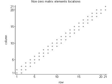
>plots[sparsematrixplot](M,title="Non-zero matrix elements locations");
>
25
>#------------------------------------------------------
>L_x:=[seq((i-1)*dx,i=1..Nx)]:
>#---------------------------------
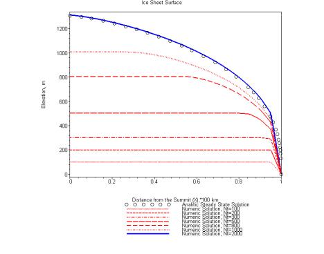
>gr0:=plot(Sa*Zo,x=0..1,numpoints=20,color=black,style=point,sym bol=circle,symbolsize=18,legend="Analitic Steady State Solution"):
>L_S:=[seq(S1[i]*Zo,i=1..Nx)]: Surf:=spline(L_x,L_S,x,1): gr1:=plot(Surf,x=0..1,numpoints=30,color=red,thickness=2,linestyle= 2,legend="Numeric Solution, Nt=100"):
>L_S:=[seq(S2[i]*Zo,i=1..Nx)]: Surf:=spline(L_x,L_S,x,1): gr2:=plot(Surf,x=0..1,numpoints=30,color=red,thickness=2,linestyle= 3,legend="Numeric Solution, Nt=200"):
>L_S:=[seq(S3[i]*Zo,i=1..Nx)]: Surf:=spline(L_x,L_S,x,1): gr3:=plot(Surf,x=0..1,numpoints=30,color=red,thickness=2,linestyle= 4,legend="Numeric Solution, Nt=300"):
>L_S:=[seq(S4[i]*Zo,i=1..Nx)]: Surf:=spline(L_x,L_S,x,1): gr4:=plot(Surf,x=0..1,numpoints=30,color=red,thickness=2,linestyle= 5,legend="Numeric Solution, Nt=500"):
>L_S:=[seq(S5[i]*Zo,i=1..Nx)]: Surf:=spline(L_x,L_S,x,1): gr5:=plot(Surf,x=0..1,numpoints=30,color=red,thickness=2,linestyle= 6,legend="Numeric Solution, Nt=800"):
>L_S:=[seq(S6[i]*Zo,i=1..Nx)]: Surf:=spline(L_x,L_S,x,1): gr6:=plot(Surf,x=0..1,numpoints=30,color=red,thickness=3,linestyle= 7,legend="Numeric Solution, Nt=1000"):
>L_S:=[seq(S[i]*Zo,i=1..Nx)]: Surf:=spline(L_x,L_S,x,1): gr7:=plot(Surf,x=0..1,numpoints=30,color=blue,thickness=3,linestyle =1,legend="Numeric Solution, Nt=2000"):
plots[display]([gr0,gr1,gr2,gr3,gr4,gr5,gr6,gr7],axes=boxed,title="Ice Sheet Surface",labels=["Distance from the Summit (X),*100 km","Elevation, m"],labeldirections=[HORIZONTAL,VERTICAL]);
26
>#-------------------------------------------------------------
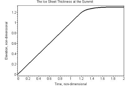
>L_t:=[seq(m*dt,m=0..Nt)]:
>L_S:=[seq(H_Ice_Summit[m],m=0..Nt)]:
>Surf:=spline(L_t,L_S,t,1):
>plot(Surf,t=0..Nt*dt,numpoints=10,axes=boxed,title="The Ice Sheet Thickness at the Summit", labels=["Time, nondimensional","Elevation, nondimensional"],labeldirections=[HORIZONTAL,VERTICAL],color= black,thickness=3,linestyle=1);
27
>#-------------------------------------------------------------------
>#--------- The full time of the ice accumulation ----------
>#-------------------------------------------------------------------
>T_accumulation:=To*1.8;
T_accumulation := 6042.040164
Дополнение. Примеры неустойчивости схемы.
>#+++++++++++++++++++++++++++++++++++++++++++++++
>#+++++++ The examples of the model instability +++++++++++
>#+++++++++++++++++++++++++++++++++++++++++++++++
>#-- dt:=0.02: Nx:=8: --
28

> #--- dt:=0.01: Nx:=11: ---
>
29
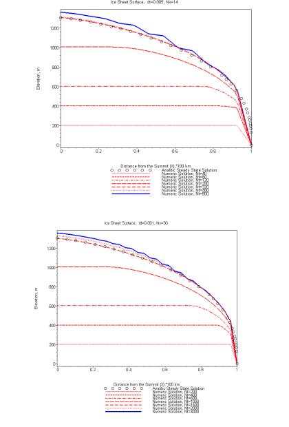
> #--- dt:=0.005: Nx:=14: ---
> #--- dt:=0.001: Nx:=30: ---
30