96	The Scientist and Engineer's Guide to Digital Signal Processing

Special Properties of Linearity

Linearity is commutative, a property involving the combination of two or more systems. Figure 5-10 shows the general idea. Imagine two systems combined in a cascade, that is, the output of one system is the input to the next. If each system is linear, then the overall combination will also be linear. The commutative property states that the order of the systems in the cascade can be rearranged without affecting the characteristics of the overall combination. You probably have used this principle in electronic circuits. For example, imagine a circuit composed of two stages, one for amplification, and one for filtering. Which is best, amplify and then filter, or filter and then amplify? If both stages are linear, the order doesn't make any difference and the overall result is the same. Keep in mind that actual electronics has nonlinear effects that may make the order important, for instance: interference, DC offsets, internal noise, slew rate distortion, etc.

FIGURE 5-7

The commutative property for linear systems. When two or more linear systems are arranged in a cascade, the order of the systems does not affect the characteristics of the overall combination.

IF

x[n]	System	System	y[n]
	A	B

THEN
x[n]	System	System	y[n]
	B	A

Figure 5-8 shows the next step in linear system theory: multiple inputs and outputs. A system with multiple inputs and/or outputs will be linear if it is composed of linear subsystems and additions of signals. The complexity does not matter, only that nothing nonlinear is allowed inside of the system.

To understand what linearity means for systems with multiple inputs and/or outputs, consider the following thought experiment. Start by placing a signal on one input while the other inputs are held at zero. This will cause the multiple outputs to respond with some pattern of signals. Next, repeat the procedure by placing another signal on a different input. Just as before, keep all of the other inputs at zero. This second input signal will result in another pattern of signals appearing on the multiple outputs. To finish the experiment, place both signals on their respective inputs simultaneously. The signals appearing on the outputs will simply be the superposition (sum) of the output signals produced when the input signals were applied separately.

FIGURE 5-8

Any system with multiple inputs and/or outputs will be linear if it is composed of linear systems and signal additions.

Chapter 5- Linear Systems

97

x1[n]	System	System	y1[n]
	A	B
x2[n]	System		y2[n]
	C
x3[n]	System	System	y3[n]
	D	E

The use of multiplication in linear systems is frequently misunderstood. This is because multiplication can be either linear or nonlinear, depending on what the signal is multiplied by. Figure 5-9 illustrates the two cases. A system that multiplies the input signal by a constant, is linear. This system is an amplifier or an attenuator, depending if the constant is greater or less than one, respectively. In contrast, multiplying a signal by another signal is nonlinear. Imagine a sinusoid multiplied by another sinusoid of a different frequency; the resulting waveform is clearly not sinusoidal.

Another commonly misunderstood situation relates to parasitic signals added in electronics, such as DC offsets and thermal noise. Is the addition of these extraneous signals linear or nonlinear? The answer depends on where the contaminating signals are viewed as originating. If they are viewed as coming from within the system, the process is nonlinear. This is because a sinusoidal input does not produce a pure sinusoidal output. Conversely, the extraneous signal can be viewed as externally entering the system on a separate input of a multiple input system. This makes the process linear, since only a signal addition is required within the system.

x[n]	x1[n]
y[n]	y[n]
constant	x2[n]

Linear	Nonlinear
a. Multiplication by a constant	b. Multiplication of two signals

FIGURE 5-9

Linearity of multiplication. Multiplying a signal by a constant is a linear operation. In contrast, the multiplication of two signals is nonlinear.

98	The Scientist and Engineer's Guide to Digital Signal Processing

Superposition: the Foundation of DSP

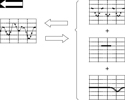
When we are dealing with linear systems, the only way signals can be combined is by scaling (multiplication of the signals by constants) followed by addition. For instance, a signal cannot be multiplied by another signal. Figure 5-10 shows an example: three signals: x0[n] , x1[n] , and x2[n] are added to form a fourth signal, x [n]. This process of combining signals through scaling and addition is called synthesis.

Decomposition is the inverse operation of synthesis, where a single signal is broken into two or more additive components. This is more involved than synthesis, because there are infinite possible decompositions for any given signal. For example, the numbers 15 and 25 can only be synthesized (added) into the number 40. In comparison, the number 40 can be decomposed into:

1 % 39 or 2 % 38 or & 30.5 % 60 % 10.5 , etc.

Now we come to the heart of DSP: superposition, the overall strategy for understanding how signals and systems can be analyzed. Consider an input

x0[n]

synthesis x[n]

decomposition

x1[n]

FIGURE 5-10

Illustration of synthesis and decomposition of signals. In synthesis, two or more signals are added to form another signal. Decomposition is the opposite process, breaking one signal into two or more additive component signals.

x2[n]

Chapter 5- Linear Systems

99

x[n]

The Fundamental

Concept of DSP

decomposition

x0[n]	System

x1[n]

System

x2[n] System

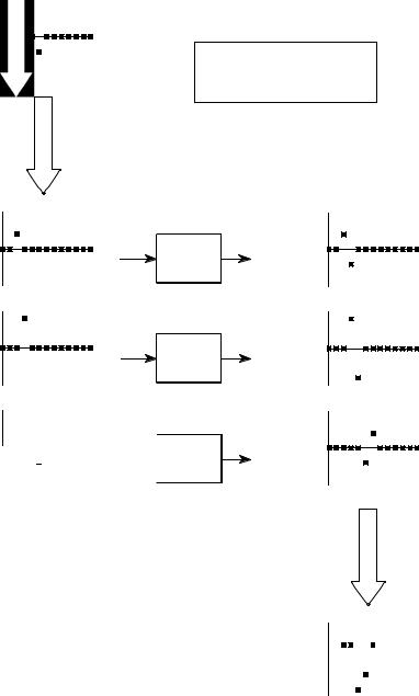
FIGURE 5-11

The fundamental concept in DSP. Any signal, such as x [n], can be decomposed into a group of additive components, shown here by the signals: x1[n], x2[n], and x3[n] . Passing these components through a linear system produces the signals, y1[n], y2[n], and y3[n] . The synthesis (addition) of these output signals forms y [n], the same signal produced when x [n] is passed through the system.

y0[n]

y1[n]

y2[n]

synthesis

y[n]

signal, called x[n] , passing through a linear system, resulting in an output signal, y[n] . As illustrated in Fig. 5-11, the input signal can be decomposed into a group of simpler signals: x0[n] , x1[n] , x2[n] , etc. We will call these the input signal components. Next, each input signal component is individually passed through the system, resulting in a set of output signal components: y0[n] , y1[n] , y2[n] , etc. These output signal components are then synthesized into the output signal, y[n] .