104	The Scientist and Engineer's Guide to Digital Signal Processing

results are dramatic; it is common for the speed to be improved by a factor of hundreds or thousands.

Fourier Decomposition

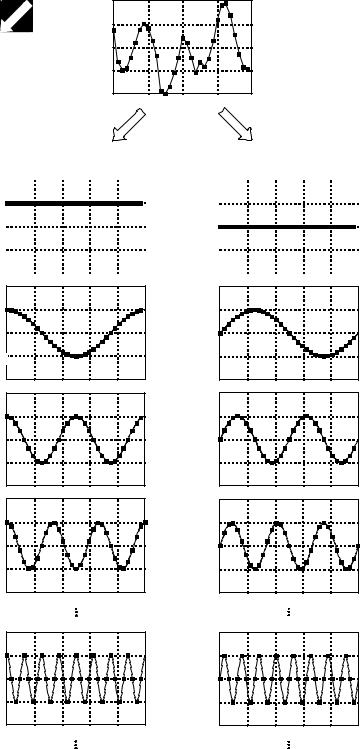
Fourier decomposition is very mathematical and not at all obvious. Figure 5-16 shows an example of the technique. Any N point signal can be decomposed into N% 2 signals, half of them sine waves and half of them cosine waves. The lowest frequency cosine wave (called xC0 [n] in this illustration), makes zero complete cycles over the N samples, i.e., it is a DC signal. The next cosine components: xC1 [n], xC2 [n], and xC3 [n], make 1, 2, and 3 complete cycles over the N samples, respectively. This pattern holds for the remainder of the cosine waves, as well as for the sine wave components. Since the frequency of each component is fixed, the only thing that changes for different signals being decomposed is the amplitude of each of the sine and cosine waves.

Fourier decomposition is important for three reasons. First, a wide variety of signals are inherently created from superimposed sinusoids. Audio signals are a good example of this. Fourier decomposition provides a direct analysis of the information contained in these types of signals. Second, linear systems respond to sinusoids in a unique way: a sinusoidal input always results in a sinusoidal output. In this approach, systems are characterized by how they change the amplitude and phase of sinusoids passing through them. Since an input signal can be decomposed into sinusoids, knowing how a system will react to sinusoids allows the output of the system to be found. Third, the Fourier decomposition is the basis for a broad and powerful area of mathematics called Fourier analysis, and the even more advanced Laplace and z-transforms. Most cutting-edge DSP algorithms are based on some aspect of these techniques.

Why is it even possible to decompose an arbitrary signal into sine and cosine waves? How are the amplitudes of these sinusoids determined for a particular signal? What kinds of systems can be designed with this technique? These are the questions to be answered in later chapters. The details of the Fourier decomposition are too involved to be presented in this brief overview. For now, the important idea to understand is that when all of the component sinusoids are added together, the original signal is exactly reconstructed. Much more on this in Chapter 8.

Alternatives to Linearity

To appreciate the importance of linear systems, consider that there is only one major strategy for analyzing systems that are nonlinear. That strategy is to make the nonlinear system resemble a linear system. There are three common ways of doing this:

First, ignore the nonlinearity. If the nonlinearity is small enough, the system can be approximated as linear. Errors resulting from the original assumption are tolerated as noise or simply ignored.

Chapter 5- Linear Systems

105

x[n]

Fourier

Decomposition

			cosine waves					sine waves
xC0[n]					xS0[n]

xC1[n]

xS1[n]

xC2[n]

xC3[n]

xS2[n]

xS3[n]

xC8[n]

xS8[n]

FIGURE 5-16

Illustration of Fourier decomposition. An N point signal is decomposed into N+2 signals, each having N points. Half of these signals are cosine waves, and half are sine waves. The frequencies of the sinusoids are fixed; only the amplitudes can change.

106	The Scientist and Engineer's Guide to Digital Signal Processing

Second, keep the signals very small. Many nonlinear systems appear linear if the signals have a very small amplitude. For instance, transistors are very nonlinear over their full range of operation, but provide accurate linear amplification when the signals are kept under a few millivolts. Operational amplifiers take this idea to the extreme. By using very high open-loop gain together with negative feedback, the input signal to the op amp (i.e., the difference between the inverting and noninverting inputs) is kept to only a few microvolts. This minuscule input signal results in excellent linearity from an otherwise ghastly nonlinear circuit.

Third, apply a linearizing transform. For example, consider two signals being multiplied to make a third: a[n] ' b[n] × c[n]. Taking the logarithm of the signals changes the nonlinear process of multiplication into the linear process of addition: log( a[n]) ' log( b[n]) % log(c[n] ) . The fancy name for this approach is homomorphic signal processing. For example, a visual image can be modeled as the reflectivity of the scene (a two-dimensional signal) being multiplied by the ambient illumination (another two-dimensional signal). Homomorphic techniques enable the illumination signal to be made more uniform, thereby improving the image.

In the next chapters we examine the two main techniques of signal processing: convolution and Fourier analysis. Both are based on the strategy presented in this chapter: (1) decompose signals into simple additive components, (2) process the components in some useful manner, and (3) synthesize the components into a final result. This is DSP.