100	The Scientist and Engineer's Guide to Digital Signal Processing

Here is the important part: the output signal obtained by this method is identical to the one produced by directly passing the input signal through the system. This is a very powerful idea. Instead of trying to understanding how complicated signals are changed by a system, all we need to know is how simple signals are modified. In the jargon of signal processing, the input and output signals are viewed as a superposition (sum) of simpler waveforms. This is the basis of nearly all signal processing techniques.

As a simple example of how superposition is used, multiply the number 2041 by the number 4, in your head. How did you do it? You might have imagined 2041 match sticks floating in your mind, quadrupled the mental image, and started counting. Much more likely, you used superposition to simplify the problem. The number 2041 can be decomposed into: 2000 % 40 % 1 . Each of these components can be multiplied by 4 and then synthesized to find the final answer, i.e., 8000 % 160 % 4 ' 8164 .

Common Decompositions

Keep in mind that the goal of this method is to replace a complicated problem with several easy ones. If the decomposition doesn't simplify the situation in some way, then nothing has been gained. There are two main ways to decompose signals in signal processing: impulse decomposition and Fourier decomposition. They are described in detail in the next several chapters. In addition, several minor decompositions are occasionally used. Here are brief descriptions of the two major decompositions, along with three of the minor ones.

Impulse Decomposition

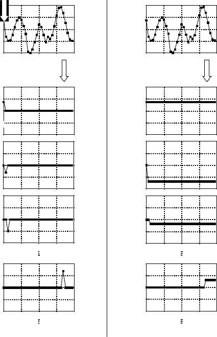
As shown in Fig. 5-12, impulse decomposition breaks an N samples signal into N component signals, each containing N samples. Each of the component signals contains one point from the original signal, with the remainder of the values being zero. A single nonzero point in a string of zeros is called an impulse. Impulse decomposition is important because it allows signals to be examined one sample at a time. Similarly, systems are characterized by how they respond to impulses. By knowing how a system responds to an impulse, the system's output can be calculated for any given input. This approach is called convolution, and is the topic of the next two chapters.

Step Decomposition

Step decomposition, shown in Fig. 5-13, also breaks an N sample signal into N component signals, each composed of N samples. Each component signal is a step, that is, the first samples have a value of zero, while the last samples are some constant value. Consider the decomposition of an N point signal, x[n] , into the components: x0[n], x1[n], x2[n], þxN& 1[n] . The k th component signal, xk[n] , is composed of zeros for points 0 through k& 1 , while the remaining points have a value of: x[k] & x[k& 1]. For example, the 5 th component signal, x5[n] , is composed of zeros for points 0 through 4, while the remaining samples have a value of: x[5] & x[4] (the difference between

Chapter 5- Linear Systems

101

x[n]

Impulse

Decomposition

x0[n]

x1[n]

x2[n]

x27[n]

FIGURE 5-12

Example of impulse decomposition. An N point signal is broken into N components, each consisting of a single nonzero point.

x[n]

Step

Decomposition

x0[n]

x1[n]

x2[n]

x27[n]

FIGURE 5-13

Example of step decomposition. An N point signal is broken into N signals, each consisting of a step function

sample 4 and 5 of the original signal). As a special case, x0[n] has all of its samples equal to x[0] . Just as impulse decomposition looks at signals one point at a time, step decomposition characterizes signals by the difference between adjacent samples. Likewise, systems are characterized by how they respond to a change in the input signal.

102	The Scientist and Engineer's Guide to Digital Signal Processing

Even/Odd Decomposition

The even/odd decomposition, shown in Fig. 5-14, breaks a signal into two component signals, one having even symmetry and the other having odd symmetry. An N point signal is said to have even symmetry if it is a mirror image around point N/2 . That is, sample x[N/2 % 1] must equal x[N/2 & 1] , sample x[N/2 % 2] must equal x[N/2 & 2] , etc. Similarly, odd symmetry occurs when the matching points have equal magnitudes but are opposite in sign, such as: x[N/2 % 1] ' & x[N/2 & 1], x[N/2 % 2] ' & x[N/2 & 2], etc. These definitions assume that the signal is composed of an even number of samples, and that the indexes run from 0 to N& 1 . The decomposition is calculated from the relations:

EQUATION 5-1

Equations for even/odd decomposition. These equations separate a signal, x [n], into its even part, xE [n] , and its odd part, xO [n] . Since this decomposition is based on circularly symmetry, the zeroth samples in the even and odd signals are calculated: xE [0] ' x [0], and xO [0] ' 0 . All of the signals are N samples long, with indexes running from 0 to N-1

x			[n ] '		x [n ] % x [N & n ]
		E
			2
x			[n ] '	x [n ] & x [N & n ]
	O
			2

This may seem a strange definition of left-right symmetry, since N/2 & ½ (between two samples) is the exact center of the signal, not N/2 . Likewise, this off-center symmetry means that sample zero needs special handling. What's this all about?

This decomposition is part of an important concept in DSP called circular symmetry. It is based on viewing the end of the signal as connected to the beginning of the signal. Just as point x[4] is next to point x[5] , point x[N& 1] is next to point x[0] . Picture a snake biting its own tail. When even and odd signals are viewed in this circular manner, there are actually two lines of symmetry, one at point x[N/2] and another at point x[0] . For example, in an even signal, this symmetry around x[0] means that point x[1] equals point x[N& 1] , point x[2] equals point x[N& 2] , etc. In an odd signal, point 0 and point N/2 always have a value of zero. In an even signal, point 0 and point N /2 are equal to the corresponding points in the original signal.

What is the motivation for viewing the last sample in a signal as being next to the first sample? There is nothing in conventional data acquisition to support this circular notion. In fact, the first and last samples generally have less in common than any other two points in the sequence. It's common sense! The missing piece to this puzzle is a DSP technique called Fourier analysis. The mathematics of Fourier analysis inherently views the signal as being circular, although it usually has no physical meaning in terms of where the data came from. We will look at this in more detail in Chapter 10. For now, the important thing to understand is that Eq. 5-1 provides a valid decomposition, simply because the even and odd parts can be added together to reconstruct the original signal.

Chapter 5- Linear Systems

103

x[n]

Even/Odd

Decomposition

even symmetry

xE[n]

	odd symmetry
xO[n]
	odd symmetry
0	N/2	N

FIGURE 5-14

Example of even/odd decomposition. An N point signal is broken into two N point signals, one with even symmetry, and the other with odd symmetry.

x[n]

Interlaced

Decomposition

even samples

xE[n]

odd samples

xO[n]

FIGURE 5-15

Example of interlaced decomposition. An N point signal is broken into two N point signals, one with the odd samples set to zero, the other with the even samples set to zero.

Interlaced Decomposition

As shown in Fig. 5-15, the interlaced decomposition breaks the signal into two component signals, the even sample signal and the odd sample signal (not to be confused with even and odd symmetry signals). To find the even sample signal, start with the original signal and set all of the odd numbered samples to zero. To find the odd sample signal, start with the original signal and set all of the even numbered samples to zero. It's that simple.

At first glance, this decomposition might seem trivial and uninteresting. This is ironic, because the interlaced decomposition is the basis for an extremely important algorithm in DSP, the Fast Fourier Transform (FFT). The procedure for calculating the Fourier decomposition has been known for several hundred years. Unfortunately, it is frustratingly slow, often requiring minutes or hours to execute on present day computers. The FFT is a family of algorithms developed in the 1960s to reduce this computation time. The strategy is an exquisite example of DSP: reduce the signal to elementary components by repeated use of the interlace transform; calculate the Fourier decomposition of the individual components; synthesize the results into the final answer. The