Finkenzeller K.RFID handbook.2003

106	4 PHYSICAL PRINCIPLES OF RFID SYSTEMS

200

|Z1| arg(Z1)

150

100

50

0	1 × 107	1.5 × 107	2 × 107	2.5 × 107
5 × 106

Figure 4.48 The measurement of impedance and phase at the measuring coil permits no conclusion to be drawn regarding the frequency of the transponder

in the form of a line diagram it has a curved path, as shown in Figure 4.48. As the measuring frequency rises the line diagram passes through various local maxima and minima for the magnitude and phase of Z1. The sequence of the individual maxima and minima is always the same.

In the event of mutual inductance with a transponder the impedance Z1 of the coupling coil L1 is made up of several individual impedances:

Z1 = R1 + j ωL1 + ZT

(4.58)

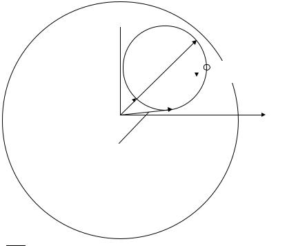
Apart from at the transponder resonant frequency fRES, ZT tends towards zero, so Z1 = RL + j ωL1. The locus curve in this range is a line parallel to the imaginary y axis of the complex Z plane at a distance of R1 from it. If the measuring frequency approaches the transponder resonant frequency this straight line becomes a circle as a result of the influence of ZT. The locus curve for this is shown in Figure 4.49. The transponder resonant frequency corresponds with the maximum value of the real component of Z1 (however this is not visible in the line diagram shown in Figure 4.48). The appearance of the individual maxima and minima of the line diagram can also be seen in the locus curve. A precise measurement of the transponder resonant frequency is therefore only possible using measuring devices that permit a separate measurement of R and X or can display a locus curve or line diagram.

4.1.12 Magnetic materials

Materials with a relative permeability >1 are termed ferromagnetic materials. These materials are iron, cobalt, nickel, various alloys and ferrite.

4.1 MAGNETIC FIELD

107

150

180

210

90

120

Im in Ω 150

100

50

Minimum value Z(f ) 0

Minimum angle Z(f )

60
			Maximum value
			30
				Resonant frequency fRES
fmess				of the transponders
				Re in Ω
			0

330

240	300
Z(f )	270

Figure 4.49 The locus curve of impedance Z1 in the frequency range 1–30 MHz

4.1.12.1Properties of magnetic materials and ferrite

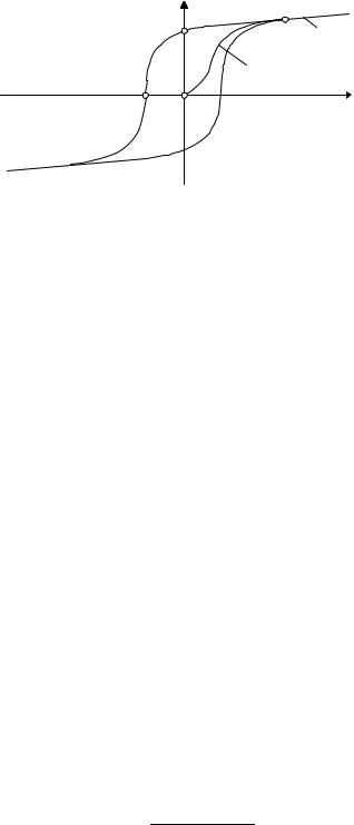
One important characteristic of a magnetic material is the magnetisation characteristic or hysteresis curve. This describes B = f (H), which displays a typical path for all ferromagnetic materials.

Starting from the unmagnetized state of the ferromagnetic material, the virgin curve A → B is obtained as the magnetic field strength H increases. During this process, the molecular magnets in the material align themselves in the B direction. (Ferromagnetism is based upon the presence of molecular magnetic dipoles. In these, the electron circling the atomic core represents a current and generates a magnetic field. In addition to the movement of the electron along its path, the rotation of the electron around itself, the spin, also generates a magnetic moment, which is of even greater importance for the material’s magnetic behaviour.) Because there is a finite number of these molecular magnets, the number that remain to be aligned falls as the magnetic field increases, thus the gradient of the hysteresis curve falls. When all molecular magnets have been aligned, B rises in proportion to H only to the same degree as in a vacuum (Figure 4.50).

When the field strength H falls to H = 0, the flux density B falls to the positive residual value BR, the remanence. Only after the application of an opposing field

108	4 PHYSICAL PRINCIPLES OF RFID SYSTEMS

B
B	Saturation
Br
Virgin curve
A
Hc	H

Figure 4.50 Typical magnetisation or hysteresis curve for a ferromagnetic material

(−H ) does the flux density B fall further and finally return to zero. The field strength necessary for this is termed the coercive field strength HC.

Ferrite is the main material used in high frequency technology. This is used in the form of soft magnetic ceramic materials (low Br), composed mainly of mixed crystals or compounds of iron oxide (Fe2O3) with one or more oxides of bivalent metals (NiO, ZnO, MnO etc.) (Vogt. Elektronik, 1990). The manufacturing process is similar to that for ceramic technologies (sintering).

The main characteristic of ferrite is its high specific electrical resistance, which varies between 1 and 106 m depending upon the material type, compared to the range for metals, which vary between 10−5 and 10−4 m. Because of this, eddy current losses are low and can be disregarded over a wide frequency range.

The relative permeability of ferrites can reach the order of magnitude of µr = 2000. An important characteristic of ferrite materials is their material-dependent limit frequency, which is listed in the datasheets provided by the ferrite manufacturer. Above the limit frequency increased losses occur in the ferrite material, and therefore ferrite

should not be used outside the specified frequency range.

4.1.12.2 Ferrite antennas in LF transponders

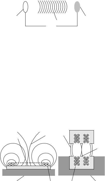
Some applications require extremely small transponder coils (Figure 4.51). In transponders for animal identification, typical dimensions for cylinder coils are d × l = 5 mm × 0.75 mm. The mutual inductance that is decisive for the power supply of the transponder falls sharply due to its proportionality with the cross-sectional area of the coil (M A; equation (4.13)). By inserting a ferrite material with a high permeability µ into the coil (M → M µ · H · A; equation (4.13)), the mutual inductance can be significantly increased, thus compensating for the small cross-sectional area of the coil.

The inductance of a ferrite antenna can be calculated according to the following equation (Philips Components, 1994):

= µ0µFerrite · n2 · A

L (4.59)

l

4.1 MAGNETIC FIELD	109

Area A	Ferrite rod
	Coil
	Length
Figure 4.51	Configuration of a ferrite antenna in a 135 kHz glass transponder

4.1.12.3Ferrite shielding in a metallic environment

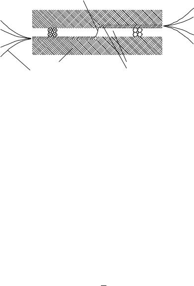
The use of (inductively coupled) RFID systems often requires that the reader or transponder antenna be mounted directly upon a metallic surface. This might be the reader antenna of an automatic ticket dispenser or a transponder for mounting on gas bottles (see Figure 4.52).

However, it is not possible to fit a magnetic antenna directly onto a metallic surface. The magnetic flux through the metal surface induces eddy currents within the metal, which oppose the field responsible for their creation, i.e. the reader’s field (Lenz’s law), thus damping the magnetic field in the surface of the metal to such a degree that communication between reader and transponder is no longer possible. It makes no difference here whether the magnetic field is generated by the coil mounted upon the metal surface (reader antenna) or the field approaches the metal surface from ‘outside’ (transponder on metal surface).

By inserting highly permeable ferrite between the coil and metal surface it is possible to largely prevent the occurrence of eddy currents. This makes it possible to mount the antenna on metal surfaces.

When fitting antennas onto ferrite surfaces it is necessary to take into account the fact that the inductance of the conductor loop or coils may be significantly increased by

Ferrite	Lines of
	magnetic flux

Ferrite

Metal	Conductor loop / coil	Metal

Figure 4.52 Reader antenna (left) and gas bottle transponder in a u-shaped core with read head (right) can be mounted directly upon or within metal surfaces using ferrite shielding

110	4 PHYSICAL PRINCIPLES OF RFID SYSTEMS

the permeability of the ferrite material, and it may therefore be necessary to readjust the resonant frequency or even redimension the matching network (in readers) altogether (see Section 11.4).

4.1.12.4Fitting transponders in metal

Under certain circumstances it is possible to fit transponders directly into a metallic environment (Figure 4.53). Glass transponders are used for this because they contain a coil on a highly permeable ferrite rod. If such a transponder is inserted horizontally into a long groove on the metal surface somewhat larger than the transponder itself, then the transponder can be read without any problems. When the transponder is fitted horizontally the field lines through the transponder’s ferrite rod run in parallel to the metal surface and therefore the eddy current losses remain low. The insertion of the transponder into a vertical bore would be unsuccessful in this situation, since the field lines through the transponder’s ferrite rod in this arrangement would end at the top of the bore at right angles to the metal surface. The eddy current losses that occur in this case hinder the interrogation of a transponder.

It is even possible to cover such an arrangement with a metal lid. However, a narrow gap of dielectric material (e.g. paint, plastic, air) is required between the two metal surfaces in order to interrogate the transponder. The field lines running parallel

Figure 4.53 Right, fitting a glass transponder into a metal surface; left, the use of a thin dielectric gap allows the transponders to be read even through a metal casing (Photo: HANEX HXID system with Sokymat glass transponder in metal, reproduced by permission of HANEX Co. Ltd, Japan)

4.2 ELECTROMAGNETIC WAVES

111

Metal (steel)

Z
Y X
A super-thin gap	Tag
	Metal top (steel)

Figure 4.54 Path of field lines around a transponder encapsulated in metal. As a result of the dielectric gap the field lines run in parallel to the metal surface, so that eddy current losses are kept low (reproduced by permission of HANEX Co. Ltd, Japan)

to the metal surface enter the cavity through the dielectric gap (see Figure 4.54), so that the transponder can be read. Fitting transponders in metal allows them to be used in particularly hostile environments. They can even be run over by vehicles weighing several tonnes without suffering any damage.

Disk tags and contactless smart cards can also be embedded between metal plates. In order to prevent the magnetic field lines from penetrating into the metal cover, metal foils made of a highly permeable amorphous metal are placed above and below the tag (Hanex, n.d.). It is of crucial importance for the functionality of the system that the amorphous foils each cover only one half of the tag.

The magnetic field lines enter the amorphous material in parallel to the surface of the metal plates and are carried through it as in a conductor (Figure 4.55). At the gap between the two part foils a magnetic flux is generated through the transponder coil, so that this can be read.

4.2Electromagnetic Waves

4.2.1The generation of electromagnetic waves

Earlier in the book we described how a time varying magnetic field in space induces an electric field with closed field lines (rotational field) (see also Figure 4.11). The electric field surrounds the magnetic field and itself varies over time. Due to the variation of the electric rotational field over time, a magnetic field with closed field lines occurs in

112	4 PHYSICAL PRINCIPLES OF RFID SYSTEMS

Magnetic field lines

Metal cover				Coil of the disk tag
Magnetic field lines				Amorphous metal

Figure 4.55 Cross-section through a sandwich made of disk transponder and metal plates. Foils made of amorphous metal cause the magnetic field lines to be directed outwards

space (rotational field). It surrounds the electric field and itself varies over time, thus generating another electric field. Due to the mutual dependence of the time varying fields there is a chain effect of electric and magnetic fields in space (Fricke et al., 1979).

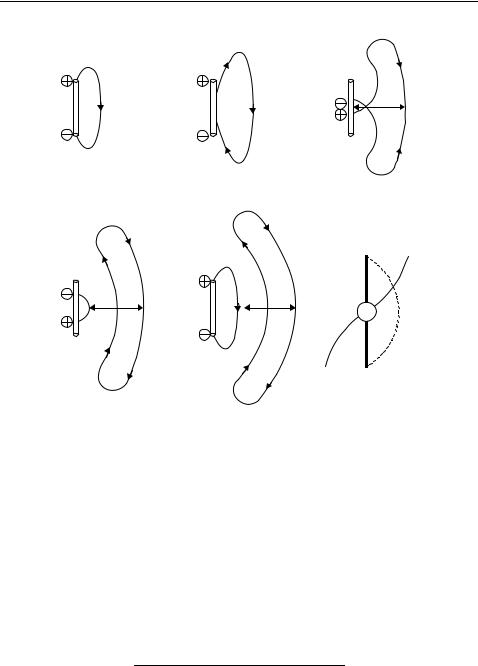
Radiation can only occur given a finite propagation speed (c ≈ 300 000 km/s; speed of light ) for the electromagnetic field, which prevents a change in the voltage at the antenna from being followed immediately by the field in the vicinity of the change. Figure 4.56 shows the creation of an electromagnetic wave at a dipole antenna. Even at the alternating voltage’s zero crossover (Figure 4.56c), the field lines remaining in space from the previous half wave cannot end at the antenna, but close into themselves, forming eddies. The eddies in the opposite direction that occur in the next half wave propel the existing eddies, and thus the energy stored in this field, away from the emitter at the speed of light c. The magnetic field is interlinked with the varying electrical field that propagates at the same time. When a certain distance is reached, the fields are released from the emitter, and this point represents the beginning of electromagnetic radiation (→ far field). At high frequencies, that is small wavelengths, the radiation generated is particularly effective, because in this case the separation takes place in the direct vicinity of the emitter, where high field strengths still exist (Fricke et al., 1979).

The distance between two field eddies rotating in the same direction is called the wavelength λ of the electromagnetic wave, and is calculated from the quotient of the speed of light c and the frequency of the radiation:

c
λ = f	(4.60)

4.2.1.1Transition from near field to far field in conductor loops

The primary magnetic field generated by a conductor loop begins at the antenna (see also Section 4.1.1.1). As the magnetic field propagates an electric field increasingly also develops by induction (compare Figure 4.11). The field, which was originally purely magnetic, is thus continuously transformed into an electromagnetic field. Moreover,

4.2 ELECTROMAGNETIC WAVES		113
(a) t = 0	(b) t = T/8	(c) t = T/4

l /2

(d) t = 3T/8

(e) t = T/2

(f) Current and voltage distribution on a dipole

U

l /2

l /2

fG

I

Figure 4.56 The creation of an electromagnetic wave at a dipole antenna. The electric field E is shown. The magnetic field H forms as a ring around the antenna and thus lies at right angles to the electric field

at a distance of λ/2π the electromagnetic field begins to separate from the antenna and wanders into space in the form of an electromagnetic wave. The area from the antenna to the point where the electromagnetic field forms is called the near field of the antenna. The area after the point at which the electromagnetic wave has fully formed and separated from the antenna is called the far field.

A separated electromagnetic wave can no longer retroact upon the antenna that generated it by inductive or capacitive coupling. For inductively coupled RFID systems this means that once the far field has begun a transformer (inductive) coupling is no

Table 4.5 Frequency and wavelengths of different VHF–UHF frequencies

Frequency	Wavelength (cm)
433 MHz	69 (70 cm band)
868 MHz	34
915 MHz	33
2.45 GHz	12
5.8 GHz	5.2

114		4 PHYSICAL PRINCIPLES OF RFID SYSTEMS
	Table 4.6 rF and λ for different frequency ranges
	Frequency	Wavelength λ (m)	λ/2π (m)
	<135 kHz	>2222	>353
	6.78 MHz	44.7	7.1
	13.56 MHz	22.1	3.5
	27.125 MHz	11.0	1.7

Field strength H (dB A/m)

60

40

H(

x)

20

60

dB/Decade

0

−20

−40

<< Near field | Far field>>

−60

−80

20 dB/Decade

−100

−120

0.01	0.1	1	10	100	1000	10 000
			Distance (m)

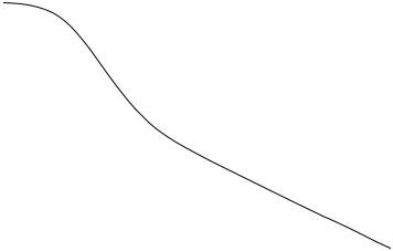
Figure 4.57 Graph of the magnetic field strength H in the transition from near to far field at a frequency of 13.56 MHz

longer possible. The beginning of the far field (the radius rF = λ/2π can be used as a rule of thumb) around the antenna thus represents an insurmountable range limit for inductively coupled systems.

The field strength path of a magnetic antenna along the coil x axis follows the relationship 1/d3 in the near field, as demonstrated above. This corresponds with a damping of 60 dB per decade (of distance). Upon the transition to the far field, on the other hand, the damping path flattens out, because after the separation of the field from the antenna only the free space attenuation of the electromagnetic waves is relevant to the field strength path (Figure 4.57). The field strength then decreases only according to the relationship 1/d as distance increases (see equation (4.65)). This corresponds with a damping of just 20 dB per decade (of distance).

4.2.2Radiation density S

An electromagnetic wave propagates into space spherically from the point of its creation. At the same time, the electromagnetic wave transports energy in the surrounding

4.2 ELECTROMAGNETIC WAVES

115

space. As the distance from the radiation source increases, this energy is divided over an increasing sphere surface area. In this connection we talk of the radiation power per unit area, also called radiation density S.

In a spherical emitter, the so-called isotropic emitter, the energy is radiated uniformly in all directions. At distance r the radiation density S can be calculated very easily as the quotient of the energy supplied by the emitter (thus the transmission power PEIRP) and the surface area of the sphere.

= PEIRP

S (4.61) 4πr2

4.2.3Characteristic wave impedance and field strength E

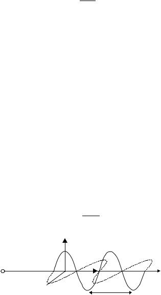
The energy transported by the electromagnetic wave is stored in the electric and magnetic field of the wave. There is therefore a fixed relationship between the radiation density S and the field strengths E and H of the interconnected electric and magnetic fields. The electric field with electric field strength E is at right angles to the magnetic field H . The area between the vectors E and H forms the wave front and is at right angles to the direction of propagation. The radiation density S is found from the Poynting radiation vector S as a vector product of E and H (Figure 4.58).

S = E × H

(4.62)

The relationship between the field strengths E and H is defined by the permittivity and the dielectric constant of the propagation medium of the electromagnetic wave. In a vacuum and also in air as an approximation:

E = H · √		= H · ZF	(4.63)
	µ0ε0

ZF is termed the characteristic wave impedance (ZF = 120π = 377 ). Furthermore, the following relationship holds:

E = S · ZF (4.64)

E

Radiation source

S

R

H

l

Figure 4.58 The Poynting radiation vector S as the vector product of E and H