funct_a_l

Chapter 1

Functions

This chapter lists and describes Mathcad’s built-in mathematical and statistical functions. The functions are listed alphabetically.

Functions labeled Professional are available only in Mathcad Professional. Certain features labeled Expert require Mathcad Professional and are available for sale separately (in Mathcad Expert Solver).

Function names are case-sensitive, but not font-sensitive. Type them in any font, but use the same capitalization as shown in the syntax section.

Many functions described here as accepting scalar arguments will, in fact, accept vector arguments. For example, while the input z for the acos function is specified as a “real or complex number,” acos will in fact evaluate correctly at each of a vector input of real or complex numbers.

Some functions don’t accept input arguments with units. For such a function f, an error message “must be dimensionless” will arise when evaluating f(x), if x has units.

Function Categories

Each function falls within one of the following categories:

•Bessel

•Complex numbers

•Differential equation solving

•Expression type

•File access

•Fourier transform

•Hyperbolic

•Interpolation and prediction

•Log and exponential

•Number theory/combinatorics

•Piecewise continuous

•Probability density

•Probability distribution

•Random number

•Regression and smoothing

•Solving

•Sorting

•Special

•Statistics

Function Categories

3

•String

•Trigonometric

•Truncation and round-off

•Vector and matrix

•Wavelet transform

The category name is indicated in the upper right corner of each entry. To see all the functions that belong to a given category, check the index of this book.

Finding More Information

You can also find information about functions using either of these methods:

•To quickly see a short description of each function from within Mathcad, choose Function from the Insert menu. Select a function in the Function field, then read the description in the Description field. Click on the Help button to see the Help topic on a selected function.

•Refer to the Resource Center QuickSheets for more detailed information about functions, categories, and related topics. Select Resource Center from the Help menu. Then click on the QuickSheets icon and select a specific topic.

About the References

References are provided in Appendix B for you to learn more about the numerical algorithm underlying a given Mathcad function or operator. References are not intended to give a description of the actual underlying source code. Some references (such as Numerical Recipes) do contain actual C code for the algorithms discussed therein, but the use of the reference does not necessarily imply that the code is what is implemented in Mathcad. The references are cited for background information only.

4	Chapter 1 Functions

Functions

acos	Trigonometric
Syntax	acos(z)
Description	Returns the inverse cosine of z (in radians). The result is between 0 and π if z is real. For complex
	z, the result is the principal value.
Arguments
z	real or complex number

acosh	Hyperbolic
Syntax	acosh(z)
Description	Returns the inverse hyperbolic cosine of z. The result is the principal value for complex z.
Arguments
z	real or complex number

acot	Trigonometric
Syntax	acot(z)
Description	Returns the inverse cotangent of z (in radians). The result is between 0 and π if z is real.
	For complex z, the result is the principal value.
Arguments
z	real or complex number

acoth	Hyperbolic
Syntax	acoth(z)
Description	Returns the inverse hyperbolic cotangent of z. The result is the principal value for complex z.
Arguments
z	real or complex number

acsc	Trigonometric
Syntax	acsc(z)
Description	Returns the inverse cosecant of z (in radians). The result is the principal value for complex z.
Arguments
z	real or complex number

Functions

5

acsch

Hyperbolic

Syntax acsch(z)

Description Returns the inverse hyperbolic cosecant of z. The result is the principal value for complex z.

Arguments

z real or complex number

Ai

(Professional)

Bessel

Syntax Ai(x)

Description Returns the value of the Airy function of the first kind.

Arguments

x real number

Example

Comments	d2	x × y = 0 .
	This function is a solution of the differential equation: ------- y –
Algorithm	dx2
	Asymptotic expansion (Abramowitz and Stegun, 1972)
See also	Bi

angle

Syntax

Description

Arguments

Trigonometric

angle(x, y)

Returns the angle (in radians) from positive x-axis to point (x, y) in x-y plane. The result is between 0 and 2p.

x, y real numbers

See also arg, atan, atan2

6	Chapter 1 Functions

APPENDPRN		File Access
Syntax	APPENDPRN( file) := A
Description	Appends a matrix A to an existing structured ASCII data file. Each row in the matrix becomes
	a new line in the data file. Existing data must have as many columns as A. The function must
	appear alone on the left side of a definition.
Arguments
file	string variable corresponding to structured ASCII data filename or path
See also	WRITEPRN for more details

arg	Complex Numbers
Syntax	arg(z)
Description	Returns the angle (in radians) from the positive real axis to point z in the complex plane. The
	result is between -p and p. Returns the same value as that of q when z is written as r × ei × q .
Arguments
z	real or complex number
See also	angle, atan, atan2

asec	Trigonometric
Syntax	asec(z)
Description	Returns the inverse secant of z (in radians). The result is the principal value for complex z.
Arguments
z	real or complex number

asech	Hyperbolic
Syntax	asech(z)
Description	Returns the inverse hyperbolic secant of z. The result is the principal value for complex z.
Arguments
z	real or complex number

Functions

7

asin	Trigonometric

Syntax asin(z)

Description Returns the inverse sine of z (in radians). The result is between −π/2 and π/2 if z is real. For complex z, the result is the principal value.

Arguments

z real or complex number

asinh

Hyperbolic

Syntax asinh(z)

Description Returns the inverse hyperbolic sine of z. The result is the principal value for complex z.

Arguments

z real or complex number

atan	Trigonometric

Syntax atan(z)

Description Returns the inverse tangent of z (in radians). The result is between −π/2 and π/2 if z is real. For complex z, the result is the principal value.

Arguments

z real or complex number

See also angle, arg, atan2

atan2

Syntax

Description

Arguments

Trigonometric

atan2(x, y)

Returns the angle (in radians) from positive x-axis to point (x, y) in x-y plane. The result is between −π and π.

x, y	real numbers
See also	angle, arg, atan
atanh	Hyperbolic
Syntax	atanh(z)
Description	Returns the inverse hyperbolic tangent of z. The result is the principal value for complex z.
Arguments
z	real or complex number

8	Chapter 1 Functions

augment

Vector and Matrix

Syntax augment(A, B)

Description Returns a matrix formed by placing the matrices A and B side by side.

Arguments

A, B two matrices or vectors; A and B must have the same number of rows

Example

See also	stack
bei	(Professional)										Bessel
Syntax	bei(n, x)
Description	Returns the value of the imaginary Bessel Kelvin function of order n.
Arguments
n	integer, n ³ 0
x	real number
Comments	The function ber(n, x) + i × bei(n, x)										is a solution of the differential equation:
	x	2	d2		d	(i × x	2	+ n	2	) × y =	0 .
			-------y + x × ----- y –
			dx	2	dx
Algorithm	Series expansion (Abramowitz and Stegun, 1972)
See also	ber
ber	(Professional)										Bessel
Syntax	ber(n, x)
Description	Returns the value of the real Bessel Kelvin function of order n.
Arguments
n	integer, n ³ 0
x	real number

Functions

9

Comments The function ber(n, x) + i × bei(n, x) is a solution of the differential equation:

	x	2	d2		d	(i × x	2	+ n	2	) × y = 0 .
			-------y + x × ----- y –
			dx	2	dx
Algorithm	Series expansion (Abramowitz and Stegun, 1972)
See also	bei
Bi	(Professional)									Bessel
Syntax	Bi(x)
Description	Returns the value of the Airy function of the second kind.
Arguments
x	real number

Comments This function is a solution of the differential equation:

d2	x × y = 0 .
------- y –
dx2

Algorithm Asymptotic expansion (Abramowitz and Stegun, 1972)

See also

Ai for example

bspline

Syntax

Description

Arguments

Interpolation and Prediction

bspline(vx, vy, u, n)

Returns the vector of coefficients of a B-spline of degree n, given the knot locations indicated by the values in u. The output vector becomes the first argument of the interp function.

vx, vy real vectors of the same size; elements of vx must be in ascending order

u real vector with n – 1 fewer elements than vx; elements of u must be in ascending order

ninteger equal to 1, 2, or 3; represents the degree of the individual piecewise linear, quadratic, or cubic polynomial fits

Comments

See also

The knots, those values where the pieces fit together, are contained in the input vector u. This is unlike traditional splines (lspline, cspline, and pspline) where the knots are forced to be the values contained in the vector vx. The fact that knots are chosen or modified by the user gives bspline more flexibility than the other splines.

lspline for more details

10	Chapter 1 Functions

bulstoer	(Professional)	Differential Equation Solving
Syntax	bulstoer(y, x1, x2, acc, D, kmax, save)
Description	Solves a differential equation using the smooth Bulirsch-Stoer method. Provides DE solution
	estimate at x2.
Arguments	Several arguments for this function are the same as described for rkfixed.
y	real vector of initial values
x1, x2	real endpoints of the solution interval
acc	real acc > 0 controls the accuracy of the solution; a small value of acc forces the algorithm to
	take smaller steps along the trajectory, thereby increasing the accuracy of the solution. Values
	of acc around 0.001 will generally yield accurate solutions.
D(x, y)	real vector-valued function containing the derivatives of the unknown functions
kmax	integer kmax > 0 specifies maximum number of intermediate points at which the solution is
	approximated; places an upper bound on the number of rows of the matrix returned by these
	functions
save	real save > 0 specifies the smallest allowable spacing between values at which the solutions are
	approximated; places a lower bound on the difference between any two numbers in the first
	column of the matrix returned by the function
Comments	The specialized DE solvers Bulstoer, Rkadapt, Stiffb, and Stiffr provide the solution y(x) over
	a number of uniformly spaced x-values in the integration interval bounded by x1 and x2. When
	you want the value of the solution at only the endpoint, y(x2), use bulstoer, rkadapt, stiffb, and
	stiffr instead.
Algorithm	Adaptive step Bulirsch-Stoer method (Press et al., 1992)
See also	rkfixed, a more general differential equation solver, for information on output and arguments.
Bulstoer	(Professional)	Differential Equation Solving
Syntax	Bulstoer(y, x1, x2, npts, D)
Description	Solves a differential equation using the smooth Bulirsch-Stoer method. Provides DE solution at
	equally spaced x-values by repeated calls to bulstoer.
Arguments	All arguments for this function are the same as described for rkfixed.
y	real vector of initial values
x1, x2	real endpoints of the solution interval
npts	integer npts > 0 specifies the number of points beyond initial point at which the solution is to be
	approximated; controls the number of rows in the matrix output
D(x,y)	real vector-valued function containing the derivatives of the unknown functions

Functions

11

Comments When you know the solution is smooth, use the Bulstoer function instead of rkfixed. The Bulstoer function uses the Bulirsch-Stoer method which is slightly more accurate under these circumstances than the Runge-Kutta method used by rkfixed.

Algorithm Fixed step Bulirsch-Stoer method with adaptive intermediate steps (Press et al., 1992)

See also rkfixed, a more general differential equation solver, for information on output and arguments.

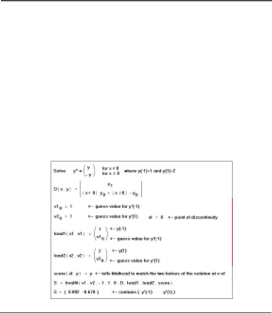
bvalfit

Syntax

Description

Arguments

(Professional)

Differential Equation Solving

bvalfit(v1, v2, x1, x2, xf, D, load1, load2, score)

Converts a boundary value differential equation to initial/terminal value problems. Useful when derivatives have a single discontinuity at an intermediate point xf.

v1	real vector containing guesses for initial values left unspecified at x1
v2	real vector containing guesses for initial values left unspecified at x2
x1, x2	real endpoints of the interval on which the solution to the DEs are evaluated
xf	point between x1 and x2 at which the trajectories of the solutions beginning at x1 and those
	beginning at x2 are constrained to be equal
D(x, y)	real n-element vector-valued function containing the derivatives of the unknown functions
load1(x1, v1)	real vector-valued function whose n elements correspond to the values of the n unknown functions
	at x1. Some of these values are constants specified by your initial conditions. If a value is
	unknown, you should use the corresponding guess value from v1
load2(x2, v2)	analogous to load1 but for values taken by the n unknown functions at x2
score(xf, y)	real n-element vector-valued function used to specify how you want the solutions to match at xf
	One usually defines score(xf, y) := y to make the solutions to all unknown functions match up at xf

Example

12	Chapter 1 Functions