Antennas

217

9.4 Dipole and Monopole Antennas

Wire antennas are popular at frequencies below 1 GHz. The dipole antenna is the most often used wire antenna. It is a straight wire, which is usually split in the middle so that it can be fed by a transmission line.

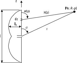
It can be thought that a dipole shown in Figure 9.7 consists of current elements in a line. The far field is calculated by summing the fields produced by the current elements, that is, by integrating (9.20):

		l /2	I (z ) e −jkR (z )
Eu =	jvm	E
				sin u(z ) dz	(9.24)
	4p		R (z )

−l /2

where l is the length of the dipole. It can be assumed that the current distribution I (z ) is sinusoidal and at the ends of the wire the current is zero. This assumption applies well for a thin wire. The current distribution can be considered to be a standing wave pattern, which is produced as the current wave reflects from the end of the wire. The current distribution is

I (z ) =	I0	sin [k (l /2 − z )],	for z > 0
	HI0	sin [k (l /2 + z )],	(9.25)
			for z < 0

where I 0 is the maximum P (r , u, f) it applies u (z )

current. Far away from the antenna at a point ≈ u and 1/R (z ) ≈ 1/r , so these terms can be

Figure 9.7 Dipole antenna.

218 Radio Engineering for Wireless Communication and Sensor Applications

assumed to be constant in (9.24). However, small changes in R (z ) as a function of z have to be taken into account in the phase term e −jkR (z ). The distance from P to the element is

R (z ) = √		≈ r − z cos u
	r 2 + z 2 − 2rz cos u		(9.26)

From (9.24), the field radiated by the dipole is

					cos S	1	kl cos uD − cos S	1	kl D
Eu =	jhI0		e	−jkr		2		2			(9.27)
	2pr						sin u

If the dipole is short compared to a wavelength, the current distribution is approximately triangular. Its radiation resistance is a quarter of that of the Hertz dipole having the same length:

Sl D

R r ≈ 20p 2

l 2

V

(9.28)

This is valid up to about a length of l

= l/4.

The half-wave dipole is the most important of dipole antennas. When

l = l/2, it follows from (9.27) that

cos S

p

cos uD

Eu =

jhI0

e

−jkr

2

(9.29)

2pr

sin u

The maximum of the field is in the plane perpendicular to the wire and the nulls are along the direction of the wire. The half-power beamwidth is u3dB = 78°. The directivity is D = 1.64 (2.15 dB), which is also the gain G for a lossless half-wave dipole. The directional patterns of the half-wave dipole and the Hertz dipole (u3dB = 90°, D = 1.5) are compared in Figure 9.8. The radiation resistance of the half-wave dipole is R r = 73.1V in a lossless case. The input impedance also includes some inductive reactance. The impedance could be made purely resistive by reducing the length of the wire by a few percent; this will reduce the radiation resistance too. In practice, the properties of the half-wave dipole also depend on the thickness of the wire.

Antennas

219

Figure 9.8 Normalized directional patterns of the half-wave and Hertz dipole.

Figure 9.9 shows a folded dipole. Both of the half-wave-long wires have a similar current distribution. Therefore, the folded dipole produces a field twice of that of the half-wave dipole for a given feed current. Thus, the radiated power is four times that of the half-wave dipole and the radiation resistance is about 300V. A parallel-wire line having a characteristic impedance of 300V is suitable for feeding a folded dipole antenna.

If a dipole antenna has a length of a few half-wavelengths, its directional pattern has several lobes. Figure 9.10 shows the current distribution and directional pattern of a 3l/2-long dipole. As the length l further increases,

Figure 9.9 Folded dipole antenna.

Figure 9.10 A 3l /2-long dipole antenna: current distribution and directional pattern.

220 Radio Engineering for Wireless Communication and Sensor Applications

the number of lobes increases. The envelope of the lobes forms a cylinder around the z -axis. The feed point of a dipole antenna is usually in the middle but can be at some other point. The directional pattern and impedance depend on the position of the feed point.

Example 9.2

Let us consider two dipole antennas having lengths of 0.1l and 0.5l . Both have a feed current of 1A. What are the radiated powers?

Solution

From (9.28), the radiation resistance is R r = 1.97V as l = 0.1l. The radiated power P = 1⁄2 R r I 2 = 1.0W. For the half-wave dipole, R r = 73.1V and P = 36.5W. Thus, a short dipole is ineffective and its small resistance is difficult to match to a transmission line.

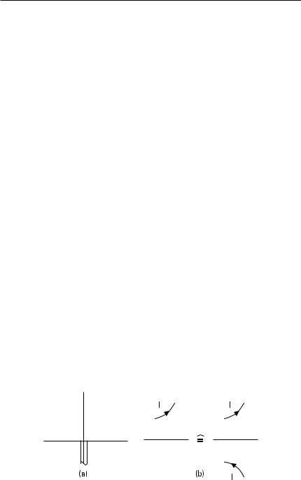
The monopole antenna is a straight wire above a ground plane as shown in Figure 9.11(a). In the analysis, the image principle can be applied. The conducting plane can be removed if an image of the current distribution is placed on the other side of the plane, as in Figure 9.11(b). This way the tangential electric field vanishes at the plane where the conducting plane was.

The monopole antenna and the dipole antenna formed according to the image principle have similar fields in the half-space above the ground plane. For a given feed current, the power radiated by the monopole is half of that of the corresponding dipole because the monopole produces no fields below the ground plane. Therefore, the radiation resistance of a quarterwave monopole is 36.5V, which is half of that of a half-wave dipole. The gain of the monopole is twice of that of the dipole.

In practice, the ground plane of a monopole antenna is finite and has a finite conductivity. Therefore, the main lobe is tilted upward and there

Figure 9.11 (a) Monopole antenna; and (b) image principle.

Antennas

221

may be a null along the direction of the surface. At low frequencies, a flat ground acts as a ground plane. The conductivity may be improved by introducing metal wires into the ground.

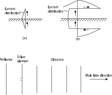
Monopole antennas operating at VLF and LF ranges are short compared to a wavelength and have a low radiation resistance. Their efficiency can be improved by adding a horizontal wire at the top, as shown in Figure 9.12. Due to the top loading, the current in the vertical part is increased. The fields produced by the vertical part and its image add constructively. However, the fields from the horizontal part and its image cancel each other, because their currents flow to opposite directions and their distance is small compared to a wavelength.

Dipole and monopole antennas are omnidirectional in the plane perpendicular to the wire and thus have a low directivity. Figure 9.13 shows a Yagi (or Yagi-Uda) antenna, which is an antenna commonly used for TV reception. It consists of an array of parallel dipoles, which together form a directional antenna. Only one element, the driven element, is fed from the transmission line. There is a reflector behind the driven element and directors in front of it. Currents are induced to these parasitic elements. The fields

Figure 9.12 (a) Short monopole antenna; and (b) top-loaded monopole antenna.

Figure 9.13 Yagi antenna.