Fundamentals of the Physics of Solids / 15-Elementary Excitations in Magnetic Systems

15

Elementary Excitations in Magnetic Systems

In the previous chapter we became acquainted with magnetically ordered materials, as well as the simple description of their behavior based on the mean-field theory. The essential point was to consider only the thermal average of atomic magnetic moments and to ignore thermal and quantum fluctuations. We noted that in the vicinity of the critical point a physically as well as mathematically correct description of critical phenomena is possible only if thermal fluctuations are taken into account, and we outlined the basics of the appropriate scaling theory and of the renormalization-group transformation.

However, the mean-field theory does not provide correct quantitative results at low temperatures, either. This is because in the mean-field-theoretical treatment ordered atomic magnetic moments are assumed to point rigidly in some – quite possibly site-dependent – direction, whereas, even classically, their rotation around the e ective field and the ensuing rotational degrees of freedom have to be taken into account to get a better description of the magnetic properties. This is analogous to going beyond the rigid-lattice approximation, and examining the vibrations of the ions about their equilibrium positions to understand the thermal properties of crystals. This dynamics of the spins will be examined in the present chapter. As with lattice vibrations, we shall first present a classical description of the waves formed in the system of spins, and give their quantum mechanical treatment next. We shall see that – similarly to crystalline materials, where the thermodynamic properties could be described properly with the help of the elementary excitations of bosonic character that were introduced in the quantum mechanical discussion of lattice vibrations, namely phonons – in magnetic systems, the destruction of magnetic order at finite temperature may be interpreted in terms of a gas of bosonic elementary excitations. At the end of the chapter we shall briefly discuss the anomalous behavior of low-dimensional magnetic systems, too.

516 15 Elementary Excitations in Magnetic Systems

15.1 Classical Spin Waves

In the mean-field-theoretical description the e ective field (14.4.4) acts on the spins. It was also assumed there that the spins or magnetic moments point exactly in the direction determined by the e ective field. In reality, this assumption is not justified within the classical framework, either. The fact that the thermal average of atomic moments decreases with increasing temperature should be interpreted like this: the moments turn slightly away from and precess about the direction of the internal e ective magnetic field, while the component perpendicular to the field averages out to zero. To illustrate this precessional motion, we shall examine the equation of motion of atomic magnetic moments that we regard as classical vectors.

15.1.1 Ferromagnetic Spin Waves

According to classical mechanics and electrodynamics, the torque experienced by a magnetic moment μ placed in a magnetic field B is μ × B, while the rate of change of the angular momentum I is given by

dI	= μ × B .	(15.1.1)
dt

We shall apply this formula to the magnetic moment μi at lattice site Ri that possesses an angular momentum Si and feels an e ective field Be. The classical equation of motion of this spin is

	dSi	= μi × Be = gμB Si × Be .	(15.1.2)
	dt

Using the formula (14.4.4) for the e ective field, assuming zero applied field, and substituting the classical vector for the average (since the equation is classical),

	dS		2	j	Jij Sj .	(15.1.3)
	dti = Si ×

The same equation would have emerged if we had used the quantummechanical equation of motion for the operator Si,

dSi	=	i	[H, Si] ,	(15.1.4)
dt

with the Heisenberg Hamiltonian, and the commutation relations of the spin operators.

Classically, this is the equation of motion governing the precessional motion of each spin in the e ective field of its neighbors. To determine its angular frequency, assume that the spins are only slightly tilted from the equilibrium value S0 common to all lattice sites,

15.1	Classical Spin Waves 517
Si = S0 + δSi ,	(15.1.5)

where δSi is small and perpendicular to S0. Substituting this into the equation of motion, and neglecting terms of second order in δSi,

dδSi = 2 Jij [δSi × S0 + S0 × δSj ] dt

j

(15.1.6)

= 2 Jij [δSi − δSj ] × S0 .

j

In systems that are uniform in the ground state, this precessional motion is expected to propagate in a wave-like fashion, therefore solutions are sought in the form

δSi = 12 Akei(k·Ri −ωk t) + Ake−i(k·Ri −ωk t)

.(15.1.7)

Inserting this into the equation of motion, we are led to

−i ωkAk = 2	j	Jij 1 − eik·(Rj −Ri ) Ak × S0 ,	(15.1.8)

and to a similar equation for the complex conjugate amplitude. The constraints of the vector character are satisfied by choosing the amplitude Ak as

−iAk = Ak × e0 ,

(15.1.9)

where e0 is the unit vector in the direction of the magnetization, e0 = S0/S, which will be chosen as the z-axis. Since the above equation asserts that Ak is perpendicular to e0 ≡ zˆ, Ak may be written with a real Ak as

Ak = Ak (xˆ − iyˆ) ,

(15.1.10)

where xˆ and yˆ are the unit vectors in the x and y directions, respectively. Substituting this into (15.1.7) for δSi, we have

δSix = Ak cos(k · Ri − ωkt) , δSiy = Ak sin(k · Ri − ωkt) . (15.1.11)

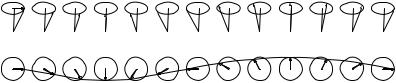
As the snapshot in Fig. 15.1 shows, the spins perform a phase-correlated precession in the plane perpendicular to the direction of the magnetization. These precessions propagating in a wave-like fashion in spin systems are called spin waves.

Going back to (15.1.8), the angular frequency of the precession of spins in the spin wave can be determined from

ωk = 2S Jij 1 − eik·(Rj −Ri ) . (15.1.12)

j

518 15 Elementary Excitations in Magnetic Systems

Fig. 15.1. The side and top views of the instantaneous orientation of classical spins in a spin-wave state

Expanding the exponent for large wavelengths, i.e. for small values of the wave number k, all odd terms cancel on account of the inversion symmetry of the lattice. In cubic crystals, where the three crystallographic axes are equivalent, the dispersion relation of the spin waves is isotropic in k space:

ωk k2 .

(15.1.13)

Similarly to the classical treatment of lattice vibrations, low-frequency vibrations are obtained in the long-wavelength limit – the only di erence being the quadratic, rather than linear frequency dependence of the wave number. This di erence – which is a consequence of the fact that the magnetization commutes with the Hamiltonian and is therefore a conserved quantity – will play an important role in the thermodynamics of the system.

15.1.2 Spin Waves in Antiferromagnets

In antiferromagnets, just like in ferromagnets, the system of magnetic moments is expected to feature propagating waves in which the precessional motion of adjacent moments follow each other by a certain phase di erence. However, because of the dissimilarity of the ground states, and since the order parameter (the sublattice magnetization) is not conserved, the dispersion relations will be essentially di erent.

We shall start o with the equation of motion (15.1.6) for the spin at site i, keeping in mind that in an antiferromagnet the spins are not all aligned in the same direction. We shall consider simple collinear structures in which case the antiferromagnetic order can be characterized by a wave vector k0, and the phase factor appearing in

Si = S0eik0·Ri

(15.1.14)

takes the values ±1 for the two possible spin orientations. Due to the precession of the spins, small time-dependent components perpendicular to the direction of S0 are superposed,

Si = Si + δSi .

(15.1.15)

Retaining only the terms that are linear in the perpendicular component, the equation of motion reads

15.1 Classical Spin Waves

519

dδSi = 2 Jij [δSi × Sj + Si × δSj ]

dt

	j		(15.1.16)
	= 2	Jij	δSi × S0eik0·Rj + S0eik0 ·Ri × δSj .
	i

Assuming periodic time dependence of angular frequency ω, orienting the z- axis along the direction of S0, and introducing the variable

Si± = δSix ± iδSiy

(15.1.17)

in the perpendicular plane, we have

±

=

2iS±

·Rj

2iSeik0·Ri

±

Jij Se

ik0

±

(15.1.18)

ωSi

i

Jij Sj .

j

j

Again, these equations can be solved using Fourier transforms. It should be noted, however, that the components k are mixed with terms of wave vector k + k0. The reason for this is that the magnetic cell of the antiferromagnetic structure is larger than the chemical cell and defines a Brillouin zone that is smaller than the usual one, therefore the vectors k and k + k0, which are not equivalent in the original Brillouin zone become equivalent in the magnetic cell. For simplicity, we are considering antiferromagnets with two sublattices in which 2k0 is identical with a vector in the reciprocal lattice of the chemical structure, and so further terms need not be taken into account.

Since the Brillouin zone contains N/2 allowed wave vectors in the twosublattice case, we shall seek solutions of the form

Si+ =	/		N		k	Ak ei(k·Ri −ωk t) + Bk ei((k−k0)·Ri −ωk t)	,
	2
Si− =	/						(15.1.19)
		N			k	Ak e−i(k·Ri −ωk t) + Bke−i((k−k0)·Ri −ωk t) .
			2

This corresponds to the assumption that the amplitude of the precessing component is |Ak +Bk| on one of the sublattices, and |Ak −Bk| on the other. Separating terms proportional to exp[±i(k·Ri−ωkt)] and exp[±i((k+k0)·Ri−ωkt)] in the equation of motion, the following relations are obtained for the coe - cients:

ωAk = ±2SBk		·(Rj −Ri ) 2SBk
	Jij eik0		Jij ei(k−k0 )·(Rj −Ri ) ,
	j		j
			(15.1.20)
ωBk = ±2SAk		·(Rj −Ri ) 2SAk
	Jij eik0		Jij eik·(Rj −Ri ) .
	j		j

Making use of the Fourier transform of the exchange interaction, the precession frequency is found to be

520 15 Elementary Excitations in Magnetic Systems
ωk = ±2S			,	(15.1.21)
	[J(k0) − J(k)][J(k0) − J(k − k0)]
where
	J(k) =	Jij eik·(Rj −Ri ) .		(15.1.22)

j

In a bipartite lattice where the nearest neighbors of each spin residing in either sublattice are located in the other sublattice, and the exchange interaction acts between nearest neighbors only,

J(k0) = z|J| and J(k − k0) = −J(k) ,

(15.1.23)

where z is the number of nearest neighbors. In this case the frequency takes the simple form

with	ωk = ±2Sω0					1 − γk2			1/2		(15.1.24)
	ω0 =			j	|Jij | = z|J|						(15.1.25)
and	Jij	eik·(Ri −Rj )					1
γk =	j | |j		|	Jij	|		=		δj	eik·δj ,	(15.1.26)
								z

where δi denotes the vectors pointing to the nearest neighbors. In the longwavelength limit γk is very close to unity, its leading correction being of the order k2. Thus, the dispersion relation of spin waves in antiferromagnetic materials is not quadratic but linear in k.

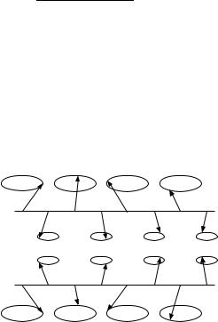
The snapshot of a propagating spin wave in antiferromagnets is shown in Fig. 15.2: spins precess with the same frequency but di erent amplitudes in the two sublattice. Because of the equivalence of the two sublattices, two types of spin waves are possible. For one, the amplitude is larger in the “up”, and for the other in the “down” sublattice.

Fig. 15.2. Propagation of the two types of spin waves in a two-sublattice antiferromagnet

15.2 Quantum Mechanical Treatment of Spin Waves

521

15.2 Quantum Mechanical Treatment of Spin Waves

Analogously to the case of phonons it may be assumed that these waves need to be quantized in the quantum mechanical treatment, in other words, that energy can change only by integral multiples of ωk. Similarly to how classical vibrations lead to phonons, classical spin waves of magnetic systems will lead to magnons. Nevertheless, there is an essential di erence: while in the quantization of lattice vibrations the canonical commutation relations for position and momentum operators implied – after the quantization of the normal coordinates – the bosonic commutation relations of phonon creation and annihilation operators, the bosonic character is only approximate for magnons, due to the special commutation relations of spin operators.

15.2.1 The Quantum Mechanics of Ferromagnetic Spin Waves

It can be easily established that the state in which the projection of each spin along a chosen direction is maximal (minimal), is an exact eigenstate of the Heisenberg Hamiltonian. To this end, consider the Hamiltonian (14.3.12) of the Heisenberg model, and choose the direction along which the spins are aligned as the quantization axis. Considering spins of magnitude S, when states with Sz = S are acted upon by the part of the Hamiltonian containing the coupling between the x and y components of the spins, the result is zero, since operators Si+ – resulting from the transcription of Six and Sjy – cannot raise the spin projection any further. The term Siz Sjz just measures the state of the spins, it does not change the spin projection. This state is an eigenstate, indeed, independently of the range and sign of the exchange interaction. Thus the energy of the state with maximum spin projection is

E = − Jij S2 .	(15.2.1)

i,j

Obviously, the state in which all spins have maximum downward projection (Sz = −S) is of the same energy. Denoting this state by |0 , and the previous one by |F , in an isotropic system, where the total spin is conserved, further states of the same energy are easily found. Two simple examples are

		√1		Si−|F and |ψ2		√1
|ψ1	=				=		Si+|0 .	(15.2.2)
		N	i			N	i

Each expression is an eigenfunction of the square of the total spin Stot =

i Si, too, with the same eigenvalue N S(N S + 1). This shows that they all represent – with di erent orientations relative to the quantization axis – the same ferromagnetic state with all spins aligned.

Further states can be generated from |ψ1 and |ψ2 when acting upon them by the same operators that generated them. These new states belong to the same eigenvalue of S2tot, that is they, too, correspond to a ferromagnetic state,

522 15 Elementary Excitations in Magnetic Systems

just the total spin is rotated relative to the quantization axis. It can be proved by the same method that the ferromagnetic state with a spin of magnitude N S is (2N S + 1)-fold degenerate. This has particular relevance when it is the ground state of the system. The condition for this is that exchange interactions be dominantly positive. Such a high degeneracy can, however, render the calculations di cult. This can be avoided by lifting the degeneracy by the application of an external magnetic field and breaking explicitly the SU(2) symmetry of the Heisenberg model; calculations are then performed in a finite field, and the results are eventually taken in the limit of vanishing field. Below, we shall follow the convention that the applied magnetic field is in the z direction, and so, if g is negative (which is often the case) the projection of each spin is −S in the ground state. We shall denote this state by |0 .

Excited states can be obtained from the ground state by flipping more and more spins, or partially raising their z-projections nonuniformly. Since spin flips are generated by the operators Si+, a general excited state is obtained by applying a series of the operators Si+ to the ground state. In the simplest case, a single spin, at lattice site Rl is raised from the state with projection −S to that with projection −S + 1. The resulting state is

|ψl = Sl+|0 .

(15.2.3)

However, this is not an eigenstate of the Heisenberg Hamiltonian. To demonstrate this, let us rewrite the Hamiltonian in terms of the spin raising and lowering operators:

−

+ S

−S+

+ Sz Sz

H = −

1

S+

−

gμ

μ H

Sz .

(15.2.4)

Jij 2

i

Sj

i j

i j

B

0

i

ij

i

If j = l, then the spin-flip terms of the type Si+Sj− can lower back the spin at Rl, while raising another spin at a di erent lattice site. Therefore, only a suitable linear combination of the states ψl with a raised spin can be a proper eigenstate. Since the eigenstates of a Hamiltonian possessing translational symmetry may be characterized by a wave vector k, we shall seek the proper eigenstate in the form

		1		√1
|ψk =	√				eik·Rl Sl+|0 .	(15.2.5)
		2S		N	l

When applying the Hamiltonian to this state, we have to separate those terms in which the projection of both spins connected by the exchange interaction is −S from those terms in which one of these spins is raised. For the latter pairs, the Siz Sjz (i = l or j = l) part of the Hamiltonian is not the only one that contributes, the Si+Sl− and Sl−Sj+ parts do so, too. Assuming that the system contains N spins, making use of the properties of the spin operators and the relation Jij = Jji , one obtains

15.2 Quantum Mechanical Treatment of Spin Waves

523

H|ψk = √2SN l					eik·Rl − i=l,j=l Jij S2 − 2 i=l						JilS(S − 1) Sl+|0
1
		2SN					−			|
+	√	1				eik·Rl		2	JilS Si+ 0		(15.2.6)
−√		1			l				i=l
						eik·Rl gμBμ0H − (N − 1)S − (S − 1) Sl+|0 .

2SN	l

Changing the summation indices in the second term, the expression chosen for the wavefunction can be recognized on the right-hand side. Consequently, the energy eigenvalue is

E = E0	+ 2S	j	Jij 1 − eik·(Ri −Rj ) − gμBμ0H ,		(15.2.7)
where
	E0 = − Jij S2 + gμBμ0HN S				(15.2.8)
				ij
is the ground-state energy. The excitation energy ωk is therefore
ωk = 2S			j	Jij 1 − eik·(Ri −Rj ) − gμBμ0H .	(15.2.9)

Aside from the second term, which is due to the magnetic field, the previous expression is analogous to (15.1.12) for the angular frequency of classical spin waves. Thus, excitation energies in the quantum mechanical treatment1 are obtained by quantizing the classically derived frequencies in the usual way.

Considering exchange interactions of strength J between nearest neighbors only, the excitation energy is customarily written as

ωk = 2JzS (1 − γk) − gμBμ0H ,

(15.2.10)

where z is the number of nearest neighbors, and γk receives its contributions from the position vectors δl of the nearest neighbors,

	1
γk =		eik·δl .	(15.2.11)
	z	δl

For a simple cubic lattice with lattice constant a, the factor z(1 − γk ) in the excitation energy is

1 − eik·δl	= 6 − 2 cos kxa − 2 cos ky a − 2 cos kz a
δl									(15.2.12)
		sin2	2	+ sin2	2		+ sin2	2
	= 4								.
			kxa		ky a			kz a

1 F. Bloch, 1930.

524 15 Elementary Excitations in Magnetic Systems

Expanding this for small values of the wave number, and then substituting back into the energy expression,

ωk ≈ 2J S kx2 + ky2 + kz2 a2 = 2J Sk2a2

(15.2.13)

is obtained in the absence of a magnetic field. The very same form applies to bodyand face-centered cubic lattices, since for a body-centered lattice

1 − eik·δl = 8 − 2 cos 12 (kx + ky + kz )a − 2 cos 12 (kx + ky − kz )a

l

−2 cos 12 (kx − ky + kz )a − 2 cos 12 (−kx + ky + kz )a

= 4 sin2

41 (kx + ky + kz )a + sin2

41 (kx + ky − kz )a

+ sin2

41 (kx − ky + kz )a + sin2

41 (−kx + ky + kz )a

≈ kx2 + ky2 + kz2

a2 = k2a2 ,

(15.2.14)

while for a face-centered lattice

1

1

1

1

1

−

eik·δl = 12

−

4 cos

1 k a

cos

1 k a

l

2

x

2

y

−

2

2

2

2

2 2

−

4 cos

2 ky a

cos

2 kz a

4 cos 2 kz a

cos 2 kxa

≈ kx + ky + kz

a

= k a .

(15.2.15)

In the long-wavelength limit, the dispersion relation of spin waves is written in the form

ωk ≈ Dk2 ,

(15.2.16)

where D is the sti ness constant of the spin waves. The experimental values for ferromagnets of the iron group are listed in Table 15.1.

Table 15.1. The experimental values of the sti ness constant for some ferromagnets

Element	Fe	Co	Ni
D/kB (10−13 K cm2)	3.32	4.66	3.99

15.2.2 Magnons as Elementary Excitations

Upon closer examination it is noted that the wavefunction (15.2.5) of the spin-wave state is created by the operator