Kosevich A.M. The crystal lattice (2ed., Wiley, 2005)(ISBN 3527405089)(342s)_PSa_

96 3 Vibrations of Polyatomic Lattices

The orthogonality and normalization properties of the functions (3.2.12), based on the conditions (3.2.11), are such that

∑msψkα (n, s)ψk α (n, s) = δkk δαα .

ns

The eigenvalues, i. e., the squared eigenfrequencies corresponding to the functions (3.2.12), are determined by the dispersion law (3.2.9). Unfortunately, a consistent analysis of the dispersion laws for a polyatomic crystal lattice that are determined as solutions to equations (3.2.9) is difficult. But we can easily perform a qualitative study where the guidelines will be the properties of vibrations in a two-component crystal model.

We proceed from the limiting case k = 0. Introduce the displacement of the center of mass of a unit cell u(n):

q	q
Mu = ∑ msus,	M = ∑ ms,	(3.2.13)
s=1	s=1
and the sum (3.2.6) over all s
ω2 Mui = ∑Assij (k)usj .		(3.2.14)
ss

We now put k = 0 on the r.h.s. of (3.2.14) and see that it vanishes due to (3.2.4)

ω2 (0)Mui = ∑Aijss (0)usj = ∑ ∑αijss (n) usj = 0. ss s ns

Thus, if u = 0 equations (3.2.6) have solutions whose frequency vanishes together with the value of the quasi-wave vector. Since there are three independent components of the unit cell center of mass there exist three branches of vibrations where, for k = 0 (λ = ∞), the unit cell of a polyatomic lattice moves as a single whole with ω = 0.

One may show that for ak 1 the linear dispersion law holds for these branches

ω(k) = sα (κ)k, κ =	k	, α = 1, 2, 3,
	k

where sα (κ) are the three sound velocities in the corresponding anisotropic medium. Thus, in a polyatomic crystal lattice there are always three acoustic branches of vibrations. The long-wave vibrations for these branches coincide with ordinary sound

vibrations of a crystal.

Equations (3.2.6) also have other solutions corresponding to ω = 0 at k = 0. In order to obtain such vibrations, we exclude from our discussion the unit cell vibrations discussed above. For this purpose, we put directly in (3.2.6) k = 0

∑Assij (0)usj = ω2 msusi ,

(3.2.15)

s

ωα (0) = ωα0

3.2 General Analysis of Vibrations of Polyatomic Lattice 97

and impose on the atom displacement the requirement
∑msus = 0.	(3.2.16)
s

It is easily seen that (3.2.16) is the compatibility condition of (3.2.15) for ω = 0. Using (3.2.16), (3.2.15) can be reduced to a set of 3q − 3 homogeneous linear alge-

braic equations to determine the same number of independent displacements. Equating the determinant of this system to zero, we obtain an equation of degree 3q − 3

relative to ω2 that yields 3q − 3 nonzero and generally different frequency values at k = 0

= 0, α = 4, 5, 6, . . . , 3q.

The frequency of these vibrations with k = 0 is nonzero because there occurs a finite relative displacement of atoms in one unit cell, requiring finite energy.

The presence of nonzero frequency for the maximum long-wave vibrations is typical for the optical branches of a crystal. Therefore, we can conclude that in a polyatomic crystal lattice there are 3q − 3 optical branches of vibrations. Since, at k = 0, the condition (3.2.16) is valid for all these vibrations the unit cell center of mass remains fixed under relevant optical vibrations. Thus, the limiting long-wave optical vibrations of a polyatomic lattice are vibrations of various monatomic sublattices (various Bravais lattices) relative to another.

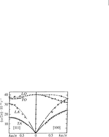
Fig. 3.2 Experimental dispersion curves of acoustic (A) and optical (O) vibrations for diamond in the directions [100] and [111] (Warren et al. 1965).

The real spectrum of vibrations of a crystal with two atoms in the unit cell is shown in Fig. 3.2, where the dispersion curves for diamond with two wave-vector directions are given. The plots show the acoustic branches (LA is the longitudinal acoustic and TA is the transverse acoustic branch) and optical branches (LO is the longitudinal optical, and TO is the transverse optical branch). Since both the chosen directions of the vector k are symmetric directions in the reciprocal lattice, all transverse modes prove to be doubly degenerate.

98 3 Vibrations of Polyatomic Lattices

In conclusion, we note that the presence of optical branches of vibrations is easily taken into account by introducing the normal coordinates of a crystal. Indeed, the transition to a polyatomic lattice is formally the adding of an extra index s (the atom number in the unit cell). The expansion of arbitrary displacements us(n) in the functions (3.2.12) remains the same as above:

us(n) = ∑Q(k, α)ψkα (n, s),	(3.2.17)
kα

where Q(k, α) are the complex normal coordinates of a polyatomic lattice. The Hamiltonian function of small crystal vibrations (2.6.8) as well as the Hamiltonian function expressed through the real normal coordinates and momenta (2.11.14) also retain their previous form. However, the summation over α is now from 1 to 3q.

3.3

Molecular Crystals

A crystal with a polyatomic lattice whose unit cell has a group of atoms interacting one with another stronger than with the atoms of neighboring groups is said to be a molecular crystal. The atoms from the chosen group are assumed to form an individual molecule, with the surrounding lattice producing an insignificant effect on its internal motion. Generally, such a crystal consists of molecules of the substance whose structure differs insignificantly from their structure in a gaseous phase. The space lattice of a molecular crystal is, as a rule, polyatomic and its unit cell often contains several molecules. Since the molecules of certain complex chemical compounds (e. g., organic ones) include a great number of atoms the linear dimension of the unit cell (identity periods) of molecular crystals may be hundreds of Angstroms.

The optical branch of molecular crystal vibrations that is responsible for intramolecular motions of strongly coupled atoms and, thus, having very high frequencies can be described as shown in Section 3.1. Such vibrations also involve the covalent atomic bonds in a molecule, and are studied as a rule independently of low-frequency types of vibrations. They represent a separate form of crystal motions and are conventionally called the internal modes of vibrations.

It is clear that the internal modes of vibrations do not exhaust all forms of motions of molecular crystals. There exist molecular motions that do not practically deform the covalent intramolecular bonds. These are the rotations of a molecule as a single whole relative to the unit cell, more exactly, around a certain crystallographic axis. These motions (“swings” of molecules) are often called librations, implying the classifications of mechanical motions of a top.

Thus, in a molecular crystal, apart from internal modes, other physically different types of motions are possible. Therefore, special terms for the corresponding vibrations are introduced. The displacements of molecular centers of mass determine the translational vibrations and the molecular librations manifest themselves in the

3.3 Molecular Crystals 99

orientational vibrations. The interaction between molecular librations is comparable in intensity with the interaction of displacements of their centers of mass. Therefore, the frequencies of the corresponding vibrations have the same order of magnitude. In other words, the orientational vibrations are not specific in terms of frequencies, but they are optically observed and, thus, specific.

In describing the vibrations of molecular crystals N2 , O2, CO2 , etc., it is assumed that rigid linear molecules are located at the lattice sites. The assumption of the rigidity of molecules means neglecting high-frequency intramolecular vibrations and allows one to represent a linear molecule as dumb-bells having two angular degrees of freedom only. There are five degrees of freedom per unit cell in such a model: the three degrees of freedom of translational vibrations described by the vector u(n) and the two degrees of freedom of librational motions that are described by two angles θ(n) and ϕ(n) that give the space orientation of linear molecules.

Restricting ourselves to a two-component model, we shall characterize a molecular state by the displacement of its center of mass u(n) and by the rotation angle around a certain axis ϕ(n). If the displacements of molecules as well as their librations are small, the linear equations for u(n) and ϕ(n) will be found by directly rewriting (3.1.3) with the replacement of ξ (n) by ϕ(n), and of the reduced mass µ by the molecular inertia moment I:

m	d2 u(n)		= − ∑ α1 (n − n )u(n ) + β(n − n )ϕ(n ) ,
	dt2
			n
			(3.3.1)
I	d2 ϕ(n)		= − ∑ α2 (n − n )ϕ(n ) + β(n − n)u(n ) .
	dt2
			n

All the results follow from (3.1.3) and discussed in Section 3.1 are automatically extended to the conclusions from (3.3.1). In particular, the dispersion relations are found as the solutions to the algebraic equation (3.1.9), where µ must be replaced by I.

Let us analyze in more detail the peculiarities of the dispersion law of a molecular crystal. Suppose the molecules are placed at the sites of a primitive cubic lattice. Now we take into account the interaction of the nearest molecules only. The nonzero elements of α(n) and β(n) matrices will then be α(0), α(n0 ) and β(0), β(n0 ), where n0 is the radius number of any one of the six nearest neighbors. We assume the matrix β(n) to be symmetric, and from (3.1.4), (3.1.10) (because the lattice is highly symmetric) we get

α1 (0) + 6α1 (n0 ) = 0; β(0) + 6β(n0 ) = 0;
α2 (0) + 6α2 (n0 ) = Iω20.	(3.3.2)

100 3 Vibrations of Polyatomic Lattices

We choose the coordinate axes along the four-fold symmetry axes and substitute (3.3.2) into (3.1.8)

A1 (k)	=	1		α1 (0)(3 − cos akx − cos aky − cos akz);
			3
B(k)	=	1		β(0)(3 − cos akx − cos aky − cos akz);			(3.3.3)
		3
				1		(α2 (0) − Iω02 )(cos akx − cos aky − cos akz ).
A2 (k)	=	α2 (0) −
					3

Using the explicit expressions (3.3.3) and solving (3.1.9), we find two dispersion relations

2mIω±2 (k) = I A1 (k) + mA2 (k)

(3.3.4)

±{[I A1 (k) − mA2 (k)]2 + 4mIB2 (k)}1/2.

We already know that for small k (ak 1) the function B2 (k) (ak)4 , and in (3.3.4) it can be omitted. The long-wave dispersion laws will then coincide with (3.1.11), (3.1.12), but we write them in a more general form

2mIω±2 (k) = I A1 (k) + mA2 (k) ± |mA2 (k) − I A1 (k)| .

(3.3.5)

Assume now that the interaction of translational and orientational vibrations is small for all k. Since the function B(k) is responsible for this interaction we omit the last term in (3.3.4), i. e., we assume that the dispersion laws are determined completely by (3.3.5). If I A1 (k) < mA2 (k) for all k, this conclusion allows one to interpret the results. The resulting dispersion laws of acoustic and optical vibrations

2

(k) =

1

A1

(k) =

α1 (0)

(3

− cos akx − cos aky − cos akz) ,

ω A

m

3m

1

α (0)

1

α (0)

ωO2 (k) =

A2

(k) =

2

=

ω02 −

2

I

I

3

I

×

(cos akx + cos aky + cos akz) ,

(3.3.6)

(3.3.7)

are described by the plots in Fig. 3.1, if the vector k is along the direction [111]. In this case the point kB corresponds to the values akx = aky = akz = π and the limiting short-wave frequencies are equal to

ωm =

2α1 (0)/m

, ω1 = (2α2 (0)/ I) − ω02 .

(3.3.8)

By assumption, ωm < ω1 (because the molecule has a small moment of inertia). The positive B2 in (3.3.4) may only decrease ωm and increase ω1. Thus, the condition

k < k < kB ,

0 < k < k ,

k < k < kB ,

3.4 Two-Dimensional Dipole Lattice 101

ωm < ω1 is not violated by taking into account the interaction of translational and orientational vibrations.

We have already noted that the characteristic frequencies of translational and librational waves have the same order of magnitude: α1 (0) mα2 (0). Hence, the crystals for which Iα1 (0) > mα2 (0) and ω1 < ωm are quite possible. The plots of the dispersion laws (3.3.6), (3.3.7) along the direction [111] will then intersect at a certain point k (Fig. 3.3a), so that a crossover situation arises. Formally, following (3.3.4), the dispersion laws of acoustic (low-frequency) and optical (high-frequency) vibrations are

1

ω2A(k) =

m A1 (k), 0 < k < k ,

1I A2 (k),

(3.3.9)

1I A2 (k),

ωO2 (k) =

m1 A1 (k),

As a result of the interaction at the point k = k , a discontinuous change in the polarizations of the vibrations of two branches occurs. Actually, it follows from (3.1.7) at B(k) = 0 that the dispersion law mω2 = A1 (k) refers to purely translational vibrations (φ = 0), and the dispersion law Iω2 = A2 (k) to the orientational vibrations (u = 0). The jump-like change in the vibration polarizations and the breaks appearing in the plots of the dispersion laws of acoustic and optical vibrations are the result of disregarding the interaction of translational and librational vibrations at Iα1 (0) > mα2 (0). The inclusion of even a small value of B2 in (3.3.4) eliminates both misunderstandings, as intersection point vanishes, the plots in the vicinity of k = k move apart, the dispersion laws become regular (Fig. 3.3b) and the polarizations transform continuously.

The above-described peculiarities of the vibration spectrum are typical for some molecular crystals mentioned above.

3.4

Two-Dimensional Dipole Lattice

A two-dimensional lattice can be made up of particles adsorbed onto an atomically smooth face of some crystals. If charged particles (ions) are adsorbed onto a metal surface each of them manifests itself as an electric dipole perpendicular to the surface. This is connected with the fact that the electrostatic charge field near the conductor (metal) plane surface is equivalent to a Coulomb charge field and its mirror reflec-

102 3 Vibrations of Polyatomic Lattices

Fig. 3.3 The “cross situation”: (a) intersection of dispersion branches; (b) removal of degeneracy.

tion in the plane surface (the opposite sign charge). Therefore, the adsorbed charged particles interact as parallel dipoles. When adsorbed particles are dense enough they are ordered and form a two-dimensional crystal that is the simplest realization of a 2D dipole lattice. The adsorbed particles, however, interact strongly enough with a substrate, such that this crystal can be regarded as two-dimensional only in terms of the geometry of its lattice.

Examples of systems whose dynamics under certain approximations are equivalent to 2D vibrations seem to be of greater interest. Under certain conditions a 2D crystal forms from electrons on a liquid helium surface at low temperatures. Electrons that have been (forced) pressed by an electric field to the liquid helium surface behave generally as a gas (gas of interacting particles), but at low enough temperatures Wigner crystallization may occur in the electron gas concerned and a 2D electron crystal appears. Electrons over the thick layer surface of dielectric helium interact almost like point charges. Thus, although the electrons on the liquid helium surface create a crystal lattice, the latter may not be a dipole. Only when a thin helium film is formed on a metal substrate is the electron interaction at large distances similar to the dipole interaction.

Finally, a 2D crystal may be formed by a system of magnetic bubbles. They can be obtained in a thin ferromagnetic film whose magnetic anisotropy axis is perpendicular to the plane of the film. In a strong enough magnetic field H directed along the normal to the film, a ferromagnetic film is in a single domain state. The magnetization M coincides in its direction with H. However, if the external field is not very strong, cylindrical “islands” where the magnetization M is directed opposite to the external magnetic field appear in the film (Fig. 3.4). These are just cylindrical magnetic domains or bubbles. They are generally observed in films of thickness 10−4 − 10−3 cm and have a diameter of the same order or even less. But in any case the bubbles prove to be macroscopic formations whose dimension is much larger than the thickness of

3.4 Two-Dimensional Dipole Lattice 103

the domain boundary dividing the regions with different orientation of magnetization. A considerable “surface” energy concentrated at the domain boundary provides a circular form of the bubble cross section.

The peculiarity of the bubbles is their great mobility and the ability to move easily along the film. But moving bubbles create around themselves a dynamical magnetization field with certain inertia. As a rule, the inertia of the inhomogeneous magnetization field is attributed, in such cases, to its source, the bubble. As a result it appears that the bubble may be regarded as some particle in a 2D crystal with the definite effective mass m . It is clear that the bubble is an isolated magnetic dipole in the background of a uniformly magnetized film (its magnetic moment equals µ = 2MhS, where h is the film thickness; S is the bubble cross-sectional area). Therefore, it is affected by the action of both inhomogeneous external magnetic field and the forces of magnetic dipole interaction with the other bubbles. The dipole interaction results in a repulsion of the same magnetic dipoles. Therefore, in a film of finite area the bubbles may form a periodic lattice. If the magnetic properties of a film are isotropic in its plane, a hexagonal (or trigonal) lattice is stable.

Let the lattice constant a be much larger that the bubble diameter (a2 S) and the plate thickness (a h). The interaction energy of two bubbles at the points R and R may then be represented as the dipole–dipole interaction energy V(R − R ), where

V(R) =	µ2
	R3 .	(3.4.1)

It is assumed in (3.4.1) that the bubble magnetic moments µ are strictly perpendicular to the plane of the film and precession deviations are absent.

Let us consider small translational vibrations1 of a bubble lattice. We introduce ui(n), i = 1, 2 as the displacement vector of a bubble located at the point with 2D number n(n1 , n2 ) that numbers unit cells. The equilibrium distance between the bubble centers in a static lattice is denoted by a.

Fig. 3.4 Distribution of magnetization in a film with bubbles.

Let the bubbles experience small displacements from the equilibrium lattice points: Rn = r(n) + u(n). Then, within the approximation quadratic in u(n) the total inter-

1) Analyzing only the vibrations of the bubble gravity centers we assume that at the frequencies we are interested in the values and the direction of a magnetic moment µ remain unchanged, the domain pulsation and precession motion of its magnetic moment do not exist, with these motions taking place at higher frequencies.

104 3 Vibrations of Polyatomic Lattices

action energy of the bubbles is given by
U =	1	∑ V(R − R ) = U0	+	1	∑	∂2 V
	2			4		∂X	∂X	k	0	(3.4.2)
		R=R				i

×[ui(n) − ui(n )] [uk (n) − uk (n )] ,

where U0 is the bubble equilibrium lattice energy.

The simplest version of the pair interaction energy (3.4.1) allows one to describe consistently the low-frequency vibrations of a dipole lattice. The expression (3.4.2) is easily reduced to a standard form (2.1.11) by denoting

αik(n) = −

αik(0) = ∑

n=0

	∂2 V		=	3µ2	r2 (n)δik − 5xi(n)xk (n) , n > 0;
	∂Xi∂Xk	0		r7 (n)		(3.4.3)
αik(n).

By calculating the elements of the matrix of atomic force constants (3.4.3), the problem of harmonic vibrations of the bubble plane lattice is actually solved.

The long-wave dipole lattice vibrations should be described by two-dimensional equations of elasticity theory of the type (2.8.6), (2.8.7), where elasticity moduli are calculated using (2.8.5), (2.8.11). With the presence of the six-fold symmetry axis (hexagonal dipole lattice), the 2D symmetrical fourth-rank tensor ciklm can be presented as (i, k = 1, 2)

ciklm = Aδ δ	+ B(δ δ	+ δ δ ).	(3.4.4)
ik lm	il km	im kl

To calculate A and B we will use (1.8.5). We will convolute over the pair of indices i and k in (2.8.5) and (3.4.4) and then over k and l. Thus, we get

A =	3µ2	Q, B =	15µ2	Q,	Q = ∑		1	.	(3.4.5)
	16		16			3	(n)
					n=0	r

In a two-dimensional lattice, the sum involved in (3.4.5) converges. Therefore, it is easily estimated by replacing the sum with a two-dimensional integral:

1

1

dx dy

1

∞

2π

Q = ∑

2πdr

=

.

r3

(n)

S0

r3

a2

r2

a3

n=0

a

Analogous to (3.4.4), the expression for a 2D tensor of elastic moduli λiklm in an hexagonal lattice can be written as (i, k = 1, 2):

λiklm = λδ δ	+ G(δ δ	+ δ δ ),	(3.4.6)
ik lm	il km	im kl

where G is the shear modulus, λ is the Lamé coefficient of a two-dimensional elastic medium. We now make use of (2.8.11) replacing V0 with S0 , the 2D lattice unit cell

3.5 Optical Vibrations of a 2D Lattice of Bubbles 105

area. We then obtain λS0 = 2B − A = 9A, GS0 = A. Thus, the elastic moduli of a 2D dipole lattice are λ = 9A/S0 2πµ2 /a5 .

Since the two-dimensional dipole lattice has both a total compression modulus and shift modulus, longitudinal and transverse elastic waves can propagate in it. The squares of longitudinal, c2l and transverse c2t , wave velocities are determined by the

formulae known from elasticity theory
c2	=	λ + 2G	S ;	c2	=	G	S .	(3.4.7)
l		m	0	t		m	0

Irrespective of specific elastic wave velocity values, the ratio of their squares in the model of a bubble lattice is given by

	cl	2
		= 11.	(3.4.8)
	ct

The number obtained is due to the choice of the pair interaction energy in the form of (3.4.1). Therefore, the relation (3.4.8) should be preserved for any plane dipole lattice of a similar type.

3.5

Optical Vibrations of a 2D Lattice of Bubbles

Using the simplest model we considered in the previous section the low-frequency (i. e., acoustic) vibrations of a 2D dipole lattice. Generalizing the model one can also study the optical vibrations of a 2D dipole lattice.

We consider two independent generalizations of the above model. First, for the bubble lattice, we take into account the magnetic domain pulsations connected with symmetric extensions and compressions of the region of “inverted” orientation of the magnetization vector M.

With existing pulsations there appears a new dynamic variable – the bubble radius

– denoted as R. Setting up the equations for the new dynamic variable, we assume as before that the bubble radius is much larger than the thickness of a domain boundary dividing the regions with opposite magnetization directions. The bubble inertia will then be concentrated almost in its cylinder surface and the surface kinetic energy can be written as (1/2)ηv2n, where η is the surface effective mass density of the domain boundary; vn is the boundary motion velocity normal to its surface (vn = dR/dt). If the bubbles move translationally with velocity V, then vn = V cos ϕ(0 < ϕ < 2π)

	and the kinetic energy of its translational motion is determined by
	Etr	= π Rhη	v2	=	π	RhV2	=	1	m V2 .	(3.5.1)
					2			2
	kin		n

If there are small pulsations under which the boundary moves uniformly at all points of the bubble surface with velocity vn = V, then the kinetic energy is given by

Epul = πηhRv2		= πηhRV2 .	(3.5.2)
kin	n