Kosevich A.M. The crystal lattice (2ed., Wiley, 2005)(ISBN 3527405089)(342s)_PSa_

1.4 Solitons of Bending Vibrations of a Linear Chain 35

Taking into account (1.4.10), (1.4.8) is simplified as

	I2
wxx +	βw2 + γ − w4 w = 0.	(1.4.11)

It is easy to see that solitary waves cannot have nonzero integral of motion I. Indeed, we set I = 0 and integrate (1.4.11)

	wx +	1	βw4	+ γw +	I2	= c, c = const.	(1.4.12)
		2			w2

It is clear that if I = 0 it is impossible to get a phase trajectory passing through a point w = wx = 0 on the phase plane at any choice of the integration constant c.

Such solutions exist only at I = 0. The case I = 0 corresponds to ϕ = const and refers to a plane-polarized bending wave running along the chain. Phase trajectories for the plane-polarized wave follow from (1.4.12)

	w2x + γw2 +	1	βw4	= c.	(1.4.13)
		2

The general behavior of the trajectories (1.4.13) is determined by the ratio of the signs of the parameters β and γ. It follows from the definition of the latter that both of them can be positive or have different signs, but cannot be negative simultaneously. Solitary waves are possible only when β > 0 and γ < 0, i. e., for V2 < ε0 . In this case there exists a typical soliton separatrix (Fig. 1.7), corresponding to c = 0, among the phase trajectories. Equation (1.4.13) at c = 0 is easily integrated

w(ξ) ≡ vx(ξ) =		2 |γ| /β				.	(1.4.14)
	cosh |γ|ξ

Fig. 1.7 Separatrix (c = 0) corresponding to a soliton.

A solitary wave of the transverse velocity field (1.4.14) is a slow soliton with velocity V < √ε0 . The absence of solitons for V > √ε0 is not surprising and is explained

36 1 Mechanics of a One-Dimensional Crystal

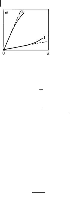
Fig. 1.8 Dispersion laws of a linear chain for the waves: 1 – bending; 2 – longitudinal.

by the form of the dispersion law for harmonic eigenvibrations of the chain. The plots of bending wave laws (Fig. 1.8 curve 1) and the longitudinal chain deformation waves (curve 2) are described√by (1.2.13) and (1.3.16).

The condition V < ε0 thus means that the soliton velocity V does not get into the interval of phase velocities of the linear chain modes and, under positive dispersion of the latter, is less than the minimum phase velocity of harmonic vibrations.

The region where the slow soliton is localized is inversely proportional to its amplitude: ∆x = 1/ |γ| = a(A/s) ε0 − V2 . For V2 → ε0 the soliton amplitude decreases proportionally to ε0 − V2 and the localization region increases as (ε0 − V2 )−1/2. It can be concluded that the soliton smears out as its velocity approaches the limiting one.

1.5

Dynamics of Biatomic 1D Crystals

A biatomic 1D crystal is different from a monatomic chain in that its unit cell contains two atoms. Let us consider the vibrations of a two-atomic 1D crystal with nearestneighbor interaction. Let atoms with masses m1 and m2 alternate, located at a distance b apart. The translational period of the crystal is a = 2b, and its lattice (Fig. 1.9) has an inversion center. Practically this is the simplest example of a superlattice consisting of two sublattices, i. e., of two Bravais lattices. Assuming the lattice point to coincide with the first atom type we obtain the following equation of motion

m1 d2 u1 (n) = −α[2u1 (n) − u2 (n) − u2 (n − 1)],

2 dt2 (1.5.1) m2 d u2 (n) = −α[2u2 (n) − u1 (n) − u1 (n + 1),

dt2

where α is a unique elastic parameter of the model.

1.5 Dynamics of Biatomic 1D Crystals 37

It is easily seen that the dispersion relation for stationary vibrations is determined

	by the solution to
	m1 ω2 − 2α			α(1 + eiak)		= 0,
	α(1 + e−iak)			m2 ω2 − 2α
	whose roots are
		1
	ω12 (k) =		ω02	1 − 1 − γ2 sin 2			ak		,
		2					2
		1							(1.5.2)
	ω22 (k) =		ω02	1 + 1 − γ2 sin 2			ak
									,
		2					2

where ω02 = 2α(m1 + m2 )/m1 m2 , γ2 = 4m1m2 /(m1 + m2 )2 .

Fig. 1.9 Diatomic one-dimensional crystal.

Therefore, every value of the quasi-wave number k meets two frequencies in the spectrum of the biatomic chain ω = ωβ(k), β = 1, 2, i. e., the dispersion relation possesses two branches of the dependence of ω on k. Two branches appear in the spectrum due to the presence of two degrees of freedom in the unit cell.

The two branches of vibrations are different. The most essential differences of the branches take place at small k(ak 1). At k = 0 we have ω1 (0) = 0, ω2 (0) = ω0 and we have in the long-wave limit (ak 1)

	1			γ2 a2
ω1 (k) = sk, s =		ω0 γa,	ω2 (k) = ω0 1 −		k2 .	(1.5.3)
	4			32

In order to formulate a difference of two types of vibrations, it is convenient to introduce the displacement of the center of mass of a pair of atoms, u(n), i. e., the center of mass of a unit cell, and the relative displacement of atoms in a pair, ξ(n):

u(n) =	1	(m1 u1 (n) + m2 u2 (n)), ξ(n) = u1 (n) − u1 (n).	(1.5.4)
	m

Under long-wave vibrations with the dispersion law ω(k) = sk, the unit cell centers of mass vibrate with the relative position of atoms in a pair remaining unchanged. Therefore, we have u(n) = u0 eiωt, ξ(n) = 0.

A feature of the second dispersion law in (1.5.3) is that the corresponding vibrations with an infinitely large wavelength have the finite frequency ω0. This vibration at

k = 0 is

u(n) = 0, ξ(n) = ξ0 e−iωt.

38 1 Mechanics of a One-Dimensional Crystal

Under such crystal vibrations the centers of mass of the unit cells are at rest and the motion in the lattice is reduced to relative vibrations inside the unit cells. The presence of such vibrations distinguishes a diatomic crystal lattice from a monatomic one.

The low-frequency branch of the dispersion law (ω < ωm) describes the acoustic vibrations, and the high-frequency one (ω1 < ω < ω2) the optical vibrations of a crystal. Thus, the biatomic 1D crystal lattice, apart from acoustic vibrations (A) also has optical vibrations (O). The optical branch of the dispersion law (1.5.2) is separated from the acoustic branch by the gap δω on the Brillouin zone boundary (Fig 1.10a), and this separation at m1 > m2 is equal:

δω = ω2 − ω1 =

2α/m2

−

2α/m1

.

(1.5.5)

Formation of a gap in 1D vibration spectrum is an inevitable consequence of the appearance of a superlattice.

The frequency ω1 = 2α/m1 is a frequency of homogeneous vibrations of the superlattice 1 relative to the resting superlattice 2, and the frequency ω2 = √2α/m2 is the frequency of homogeneous vibrations of the superlattice 2 relative the motionless superlattice 1.

However, for m1 = m2 = m the parameter γ2 = 1, the gap δω vanishes and the dispersion laws (1.5.2) degenerate:

ω1 (k) = 2

α

| sin

ak

|, ω2 (k) = 2

α

| cos

ak

| .

(1.5.6)

m

4

m

4

Fig. 1.10 Transformation of the dispersion law when the crystal period reduces twice: (a) dispersion branches at m1 = m2 , (b) junction of branches at m1 = m2.

The degeneracy corresponds to transformation of a biatomic lattice into a monatomic one with the period b = a/2. Since (1.5.6) implies that ω1 (k) = ω2 (k + (2π/a)), both equations (1.5.6) describe in fact the same acoustic dispersion law of dispersion of this 1D lattice (Fig. 1.10b).

1.6 Frenkel–Kontorova Model and sine-Gordon Equation 39

1.6

Frenkel–Kontorova Model and sine-Gordon Equation

In Section 1.2 we analyzed a deformation soliton that describes a specific elastic perturbation of the 1D crystal that belongs to the acoustic type of collective excitations, but solitary deformation waves may also arise due to the nonlinearity of optical crystal excitations.

We assume a 1D crystal to be in a given external periodic field whose period coincides with the 1D lattice constant a. The crystal energy will then be determined not only by a relative displacement of neighboring atoms, but also by an absolute displacement of separate atoms in an external potential field. We write this additional crystal energy as

W = ∑F(un), F(u + a) = F(u).	(1.6.1)
n

This situation may arise in the case when the atomic chain is on the ideally smooth surface of a 3D crystal that serves as substrate and determines a periodic potential (1.6.1).

The availability of this potential essentially affects the dynamics of a 1D system, since the equation of crystal motion now takes the form

	d2 un	= ∑α(n − n )[u(n) − u(n )] −					dF(un)
m								.	(1.6.2)
	dt2						dun
		n
If the displacements u(t) are small then
		F(u) =	1	K2 u2	,	K2 = F (0) > 0,			(1.6.3)
		2

and, thus, taking (1.6.1), (1.6.3) into account in studying small crystal vibrations

would result in the appearance in the dispersion law ω = ω(k) of a nonzero fre-

√

quency of extremely long-wave vibrations: ω(0) = ω0 = K/ m.

We shall be interested in the solutions to (1.6.2) whose behavior corresponds to the plot in Fig. 1.11 and that satisfy the boundary conditions

u(−∞) = a, u(∞) = 0.

These solutions describe such a deformation of a 1D crystal under which the atoms of the left-hand end (x = −∞) are displaced into their neighboring equilibrium positions. At x = ∞, the crystal remains undeformed u = 0, i. e., all atoms are in their positions. As the number of atoms in the crystal is fixed, the number of atoms in the vicinity of a certain point x = x0 is larger by unity than the number of the initial static equilibrium positions (Fig. 1.12).

The problem of such an aggregate of atoms near some point (a crowdion) was first considered and solved by Frenkel and Kontorova (1938), thus, the corresponding model is named after them. In the Frenkel–Kontorova model the additional assumption

40 1 Mechanics of a One-Dimensional Crystal

Fig. 1.11 Step perturbation (“overfall”) in a 1D crystal.

Fig. 1.12 Atomic distribution in a crowdion.

of a simple form of the function F(u) is made

F(u) =	1 2			2	sin	2 πu		,
		K	τ						(1.6.4)
	2						a

but the latter seems to be unimportant, although it greatly simplifies the solution to the nonlinear problem that we encounter here.

The nonlinearity of the function F(u) such as (1.6.4) is basic in the Frenkel– Kontorova model. Thus, the interatomic interaction of the nearest neighbors along a 1D crystal is sufficient to be taken into account within the harmonic approximation. In other words, the equation of crystal motion should be taken in the form

	d2 un	= α0 [un+1 + un−1 − 2un] −	aK2		2πun
m				sin		,	(1.6.5)
	dt2		2π		a

where K = πτ/a = √mω0.

Considering only the case of long waves (λ a), we go over to a continuum treatment by replacing (1.6.5) with the equation in partial derivatives

∂2 u

2 ∂2 u

a

2

2πu

2

a2 α0

= s0

−

ω0 sin

,

s0

=

.

(1.6.6)

∂t2

∂x2

2π

a

m

Equation (1.6.6) can be associated with the Lagrange function whose density is

L =

m

∂u 2

2

∂u

2

2

a 2

2 πu

− s0

− ω0

sin

.

(1.6.7)

2a

∂t

∂x

π

a

1.6 Frenkel–Kontorova Model and sine-Gordon Equation 41

In the harmonic approximation (2πu a), (1.6.6) describes optical vibrations with the dispersion law:

ω2 = ω02 + s02 k2 .

(1.6.8)

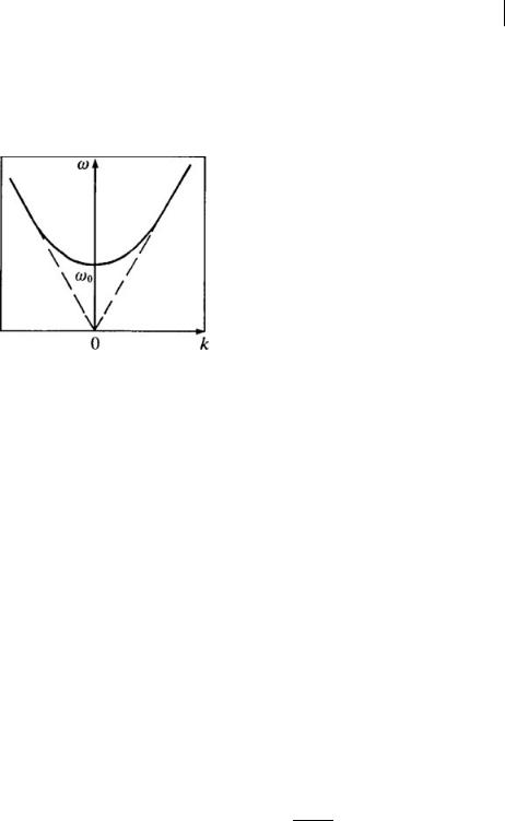
The dispersion law plot (1.6.8) is characterized by two parameters (Fig. 1.13): the limiting frequency ω0 and the minimum phase velocity of optical vibrations s0 .

Fig. 1.13 The dispersion law of harmonic vibrations.

To simplify the equations further, we introduce the dimensionless displacement 2πu/a and denote it by the same letter u. Equation (1.6.6) will then change slightly:

∂2 u	2	∂2 u	2
	= s0		− ω0 sin u.	(1.6.9)
∂t2		∂x2

This equation is called the sine-Gordon equation. All its physically meaningful solutions are now systematized and studied.

Using the results of the previous sections, we look for a solution to (1.6.9) in the form

u = u(x − Vt), V = const,

where the function u(x) satisfies the boundary conditions and has a plot such as in Fig. 1.11. The equation for the function u(x) follows from (1.6.9)

(s02 − V2 )uxx − ω02 sin u = 0.

(1.6.10)

This is actually the equation of a mathematic pendulum and can easily be integrated. The first integral of (1.6.10) corresponding to the desired function is

d2 u	= ±		2ω0			sin	u
								.	(1.6.11)
dt2							2
		2		− V	2
			s0

It is also easy to perform a second integration that leads us to the following result

	u(x, t) = 4 arctan exp	x0 − x	,	(1.6.12)
		l

42 1 Mechanics of a One-Dimensional Crystal

where l is a parameter determining the crowdion width

	2	− V	2		s0			V	2
s0
l =				=			1 −		.		(1.6.13)
	ω0				ω0			s0

When V approaches the limiting velocity s0 , the crowdion width experiences a relativistic reduction. In the limit V = s0 there arises a step with δu = a. At V = 0 a fixed inflection of width l0 = s0 /ω0 remains in the crystal.

Since a homogeneous translation onto the crystal period is a symmetry transformation, the physical state of a 1D crystal far from the point x = x0 (|x − x0 | x0 ) is similar to that in the absence of a crowdion. The derivative du/dx coinciding with a linear chain deformation is evidence of the change in the state of a one-dimensional system in the presence of a crowdion. It follows from (1.6.12) (in initial dimensional quantities)

du	= −	a			1	.	(1.6.14)
dx		πl cosh			x − x0
					l

The localized deformation (1.6.14) moving in the crystal has the form of a solitary wave and is another example of a strain soliton in a 1D crystal. Finally, coming back to a dimensional displacement and to a complete dependence on the coordinates and time in (1.6.12), we get the final expression for the displacements

u(x	t) =	2a			ω		x − Vt			(1.6.15)
		π arctan		exp −
,						0		s02 − V2 .

The perturbation described by this formula moves with velocity V (necessarily less than that of a sound s0 ). This makes it different from the shock-wave perturbation. The velocity is determined by the total energy associated with this perturbation.

The last observation will be supported with a certain qualitative argument of general character. It follows from a comparison of the properties of solitons of the two types considered by us. Irrespective of the character of nonlinearity that generates a soliton, the value of its limiting velocity is completely determined by the dispersion law of harmonic vibrations that can exist in the system under study.

If a plot of the dispersion law of linear vibrations is convex upwards similar to the plot of the dispersion law (1.2.13), it is characterized by some maximum phase velocity s0 . The velocity of a soliton (if it arises) will exceed s. If a plot of the dispersion law shows convexity downwards, as in the case of a sine-Gordon equation, it is characterized by the minimum phase velocity s0 , and the velocity of the existing soliton should be less than s0 . This conclusion will be proved in the following.

1.7 Soliton as a Particle in 1D Crystals 43

1.7

Soliton as a Particle in 1D Crystals

The local deformation associated with a crowdion (1.6.15) moved along a 1D crystal, remaining undeformed and losing no velocity, i. e., moves “by inertia” like a particle. However, the similarity between the soliton of the sine-Gordon equation and a particle is much stronger. It can be observed in the soliton dynamics in an external field.

In the long-wave approximation, the soliton energy is

		∞						∂u
E =				m
	2							∂t
	−∞
=				E0					,
						V		2
			1 −
						s0

2

+ s20

E0

	∂u 2		+ F(u)	dx
	∂x			a

	=	2	aτ√		.
				α0
		π

For small velocities (V s0 ) we have

E = m s2	+	1	m V2	,	m =	E0	=	2mτ		,
								πa√
0		2				s02			α0

(1.7.1)

(1.7.2)

where m is the effective soliton (crowdion) mass. The effective mass is less than that of an individual atom m as measured relative to the ratio of a lattice period to the rest soliton width l0 :

2a
m = m l0	m.	(1.7.3)

The energy (1.7.1) can be calculated in a standard way by means of (1.6.7) as the field energy of elastic displacement. It is natural to assume that the soliton momentum may also be determined as the momentum of the field of displacements. Then, by the definition of the field momentum,

P =

−

∂L

∂u

dx =

−

ρ

∂u

∂u

dx

,

(1.7.4)

∂ut ∂x

∂t ∂x

where ρ = m/a.

If a soliton moves with constant velocity, i. e., u(x, t) is a function of the form (1.6.15), then ∂u/∂t = −V∂u/∂x, and from (1.7.4) and (1.6.14) it follows1 that

P = ρV	∂u	2	dx = −ρ	a	2	dx			=	2ma	V.
					V
	∂x			πl		cosh2	x			π2 l
							l

1) We note that the momentum of atoms Pat is determined otherwise:

	m		∂u		m		∞			mV
Pat =								∂u
				dx = −		V			dx =		[u(−∞) − u(∞)] = mV
	a		∂t		a			∂x		a
							−∞

and equals the product of the mass of one “extra” atom m and the crowdion velocity V.

44 1 Mechanics of a One-Dimensional Crystal

Using (1.6.13) and (1.7.3), we obtain a relativistic relation between the momentum and the soliton velocity

P =		m V			.	(1.7.5)
			V	2
		1 −
			s0

Thus, the soliton behaved as a classical particle with the Hamiltonian H, where H2 = m s20 + s20 P2. For small momenta the Hamiltonian function agrees with (1.7.2)

H = E0 +	P2
	2m .	(1.7.6)

We suppose now that a 1D crystal experiences a weak external influence and denote by f (x) the density of the force acting on a 1D crystal. Equation (1.6.6) should then be replaced by

	∂2 u	2 ∂2 u			mω02		2πu	+ f (x).
ρ		= ρs0		−		sin			(1.7.7)
	∂t2		∂x2		2π		a

The long-wave approximation assumes that f (x) is a smooth function of the coordinate x varying considerably at distances large as compared to a. If the value of f (x) is small, the presence of such a perturbation in (1.7.7) cannot change considerably the soliton form, affecting mainly its dynamics. This allows us to seek a solution to (1.7.7) satisfying the boundary conditions formulated before as a soliton (1.6.15)

u(x	t) = us(x		ζ)		2a			x − ζ		(1.7.8)
		−		≡	π arctan exp		−l0
,								1 − (V/s0 )2	,

whose parameters ζ and V change slowly with the soliton moving along the crystal. Since the point x = ζ is the “center of mass” for the deformation ε(x) = ∂u/∂x, the soliton velocity may be assumed to be V = dζ/dt.

To deduce the equation determining the change in the velocity V with time, we use the following procedure. We multiply (1.7.7) by ∂u/∂x and regroup the terms in the relation obtained

∂

(utux) + ρ

∂

1

2

1 2 2

−ρ

ut +

s0 ux

∂t

∂x

2

2

(1.7.9)

+

aω0

2

2πu

1 − cos

= − f (x)ux.

2π

a

We now integrate (1.7.9) over x from −∞ to ∞ and use the definition (1.7.4) as well as the boundary conditions at infinity

	dP		∞	∂u
		= −	f (x)		dx.	(1.7.10)
	dt			∂x

−∞