Kosevich A.M. The crystal lattice (2ed., Wiley, 2005)(ISBN 3527405089)(342s)_PSa_

106 3 Vibrations of Polyatomic Lattices

Comparing (3.5.1), (3.5.2) we conclude that the effective mass of symmetric pulsations is twice as large as the effective mass of translation motion, m . Therefore, the kinetic energy of pulsations can be expressed through dR/dt in the form

Epul = m dR 2 .
kin	dt

Since the bubble pulsations change the bubble radius, they are associated with a certain increase in the potential energy of the system. Under small vibrations the potential energy of an individual bubble depends quadratically on R − R0 (R0 is the equilibrium bubble radius)

Upul = m ω2	(R	−	R	)2 ,	(3.5.3)
0			0

where ω0 is the pulsation eigenfrequency. In a lattice, the equilibrium radius R0 is different from the equilibrium radius of an isolated bubble, since the magnetodipole repulsion in a static lattice simulates a decrease in the equilibrium radius of an individual bubble.

We introduce ξ = R − R0 and calculate, in the approximation quadratic in ξ (n), the change in the magnetic-dipole interaction energy in the bubble lattice. We represent the pulsating magnetic moment of a bubble at the n-th site as

	µ(n) = µ 1 + 2	ξ	+	ξ	2
					,
				R0
		R0

where µ is an equilibrium value of the magnetic moment. Then, using (3.4.1), we write

Umd =

1

∑

µ(n)µ(n )

=

1

Nµ2 Q +

2µ2

Q ∑ξ (n)

r3 (n − n )

2

2 n=n

2

R0

(3.5.4)

2

1

2µ

ξ (n)ξ (n )

+

µ

Q ∑ ξ 2 (n) +

∑

,

R0

2

R0

n=n r3 (n − n )

where Q is determined by (3.4.5); N is the number of sites in the lattice.

The first term in (3.5.4) is included in the ground-state energy of the lattice and does not contribute to the equation of the motion for ξ (n). The second term is responsible for the renormalization of the equilibrium bubble radius. We do not give here the calculations of this renormalization (see Problem 1), keeping in mind that the equilibrium bubble radius in a lattice is different from that of an isolated bubble. The third term in (3.5.4) contributes to the renormalization of the homogeneous pulsation frequency and, finally, the fourth term determines the pulsation wave dispersion.

Using (3.5.3), (3.5.4) we introduce in a standard way the equation of motion for pulsations

2m

d2

ξ (n)

=

2m ω2

+ 2Q

µ

2

− ∑

β(n

n )ξ (n ), (3.5.5)

−

ξ (n)

−

dt2

R

0

0

n=n

3.5 Optical Vibrations of a 2D Lattice of Bubbles 107

where

β(n) =	2µ	2	1
				.
	R0		r3 (n)

Transforming (3.5.5), taking into account the definition Q, gives

m

d2

ξ (n)

=

−

m ω2

ξ (n) +

1

∑

β(n

−

n )[ξ (n)

−

ξ (n )],

dt2

2

r

n

where ωr is the renormalized pulsation frequency,

	ωr2 = ωd2 + ω02, ωd2 =	3Q µ			2
					.
		m R0

(3.5.6)

(3.5.7)

(3.5.8)

Finally, the relation (3.5.7) is written for small pulsation vibrations of the bubble lattice. For this equation the relation between the pulsations and the translational vibration of the lattice concerned was neglected. The equation for small translational vibrations was obtained, without taking into account the bubble pulsations. The relation between translational and pulsation vibrations is easily allowed for (in the expansion (3.5.4) it suffices to include the terms proportional to the bubble displacements), so the reader is invited to do this (see Problem 2).

The dispersion law for pulsation vibrations is

ω2 (k) = ωr2 −	1		∑β(n)[1 − e−ikr(n)].	(3.5.9)
	2m

It is clear that ω0 = ωr = 0. Thus, the pulsation vibrations are the optical vibrations. Furthermore, it follows from the definition (3.5.6) that β(n) > 0; hence, the second term in (3.5.9) leads to a frequency decrease with increasing k. Thus, ω = ωr is the largest frequency in the spectrum of pulsation vibrations.

Let us analyze the dispersion law (3.5.9) in the long-wavelength limit (ak 1). We denote

B(k) = ∑β(n)[e−ikr(n) − 1],

(3.5.10)

and replace the sum over the lattice with the integral in the lattice plane using the polar coordinates (r, ϕ) associated with the k vector direction

	2µ		2	1		L/2	dr			2π
B(k) =										(e−ikr cos ϕ − 1) dϕ
	R	0		S				r
				0						0
				0
	2µ		2			L/2
=				2π				dr		[ J0 (kr) − 1],
	R0			S0				r2
				0

where S0 is the unit cell area of a bubble lattice; L is the dimension (diameter) of the plane lattice; J0 (x) is the first-order Bessel function (with zero index).

108 3 Vibrations of Polyatomic Lattices

Replacing the integration variable results in

B(k) =

2µ

2 2πk

Φ

kL

,

(3.5.11)

R

0

S

0

2

where

z

1

[1 − J0

(z)] + J1

(z) − 0

J0 (x) dx.

Φ(z) =

z

Taking into account the possible values of the quasi-wave vector components (1.5.3), we conclude that the product kL either equals zero (B(0) = 0) or kL > 2π. But in the second case Φ(kL/2) does not differ in order of magnitude from its limiting value Φ(∞) = −1 and rapidly approaches it with increasing k.2 Therefore, as we are interested in the finite interval of small values k (ak 1), we can write at k = 0

B(k) =	2µ	2 2πk		Φ (∞) = −	2π 2µ			2
								k.
	R0		S0		S0		R0

Thus, the long-wave dispersion law looks like

	ω2	= ωr2		π	2µ		2
			−				k.	(3.5.12)
				m S0		R0

The frequency in (3.5.12) is independent of the direction of the 2D vector k, this being a result of the symmetry of the hexagonal lattice.

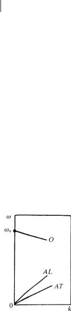
Fig. 3.5 Dispersion laws of the long-wave translational (acoustic) and pulsation (optical) vibrations of the 2D bubble lattice.

It follows from (3.5.12) that the pulsation waves for ak 1 have nonzero velocity

v = lim

∂ω

=

1 ∂B

=

π

2µ

2

−

−

,

∂k

4m ωr ∂k

2m S0 ωr

R0

k

→

0

2) The value of Φ(2π) differs from Φ(∞) = −1 by 15 per cent.

3.6 Long-Wave Librational Vibrations of a 2D Dipole Lattice 109

directed opposite to the vector k. The plots of long-wave dispersion laws of translational and pulsation waves in a bubble lattice are shown schematically in Fig. 3.5.

The dispersion law peculiarities that manifest themselves in a nonanalytic dependence of the frequency on the wave-vector components at k → 0 are due to the magnetostatic character of the dipole-interaction forces making up a lattice of bubbles.

3.6

Long-Wave Librational Vibrations of a 2D Dipole Lattice

We now proceed to the second possible generalization of a two-dimensional dipole lattice model. Assume that the centers of gravity of hard electric dipoles, oriented in the equilibrium state, perpendicular to the lattice plane (parallel to the z-axis) are fixed in the sites of a symmetric (triangular or quadratic) lattice. Each dipole can make librational vibrations and the libration frequency of an isolated dipole is equal to ω0.

If the librational vibration angles are small, the change in the z-projection of a dipole moment is of the order of its square projection onto the lattice plane. Thus, let us denote by d0 a dipole moment and let eξ be its component in the lattice plane. It then follows from the condition d2 = d20 = constant that

dz − d0 = −e2 ξ 2x + ξ 2y /2d0 eξ .

We calculate the dipole energy of the lattice in the approximation quadratic in ξ . The interaction energy of two dipoles d and d at the points n and n is equal to

	1		[R2 dd − 3(Rd)(Rd )],
	V(n − n ) =							R = r(n − n ).	(3.6.1)
		R5
	A scalar product dd in (3.6.1) for the approximation quadratic in ξ is
	d(n)d(n ) = d2			+ e2 ξ(n)ξ(n )		e2		ξ 2 (n) + ξ 2 (n ) .	(3.6.2)
					− 2d0
	0

Using (3.6.1), (3.6.2) and keeping in mind that the vector R lies in the lattice plane, we get, similar to (3.5.4), the following expression for the dipole energy

U =

1

∑V(n − n )

2

e2

=

1

d2 NQ

e2

ξ 2

(n) +

D

(n

n )ξ

(n)ξ

(n ),

2

− 2 ∑

2 ∑

ik

−

0

i

k

where Q is determined, as before, by (3.4.5), and with

Dik(n) =

1

R2 (n)δik − 3Xi(n)Xk (n) .

R5 (n)

(3.6.3)

(3.6.4)

The third term on the r.h.s. of (3.6.3) is traditional and the sign of the second term is unusual. It describes the energy decrease when dipoles deviate from the z-axis. This

110 3 Vibrations of Polyatomic Lattices

is due to the fact that at a fixed distance between the centers of two parallel dipoles, the mutual orientation along the line connecting them is the most advantageous energetically, rather than when they are perpendicular to it. But introducing the frequency ω0, we assume the presence of forces keeping the lattice in an equilibrium state with the dipoles parallel to the z-axis. The dipole interaction acts against these forces.

We now write the kinetic energy of a vibrating dipole. If we consider a dipole as a symmetric top with moment of inertia I the kinetic energy of its small librational vibrations is given by

		1		2			dξ y	2
	Ekin =		m	dξ x		+		,	(3.6.5)
		2		dt			dt

where m = e2 I/d20 α is the effective mass.

The simple form of the kinetic (3.6.5) and potential (3.6.3) energies of the lattice allows one to write down the equations of collective librational motion that take into account the dipole eigenvibrations

m	d2	ξ i(n)	= −[m ω02 − e2 Q]ξ i(n) − ∑ βik(n − n )ξ k(n ),
		dt2
			n=n

where

βik(n) = e2 Dik(n), i, k = 1, 2.

We now represent (3.6.6) in a form analogous to (3.5.7)

	d2 ξ i(n)	= −ω12	1		∑βik(n − n ) ξk(n) − ξ k(n ) ,
			ξ i(n) +
	dt2			m
					n
where						3
			ω12 = ω02 −				e2 Q.
						2m

In (3.6.8), (3.6.9) we use the relation, obvious for a symmetric lattice,

(3.6.6)

(3.6.7)

(3.6.8)

(3.6.9)

∑Dik(n) = Qδik − 3 ∑	Xi(n)Xk (n)	=	Q −	3	Q δik = −	1	Qδik.
	R5 (n)			2		2

It follows from (3.6.9) that the dipole–dipole interaction lowers the frequency of homogeneous librational vibrations of a two-dimensional dipole lattice. Since the lattice must be stable with respect to these vibrations it is necessary that ω12 > 0. In other words, the stability condition for a dipole lattice of the type concerned is given by the inequality

	3	e2 Q < ω02,	(3.6.10)
	2m

which imposes a restriction on the dipole density (i. e., on the lattice period a) since

Q 2π/a3 .

3.6 Long-Wave Librational Vibrations of a 2D Dipole Lattice 111

To analyze the dispersion law of librational vibrations we introduce the tensor functions

Bij(k) = ∑βij(n) e−ikr(n) − 1 ,

(3.6.11)

which in the long-wave approximation can be written in terms of two-dimensional space integrals. In a symmetric lattice these integrals may be calculated in a specific form of Cartesian coordinates with the x-axis directed along the vector k

Bxx(k) =		e2				dr			(1	− cos2 ϕ)[e−ikr cos ϕ − 1] dϕ,	(3.6.12)
		S				r2
	0
Byy(k) =		e2				dr			(1	− 3 sin2 ϕ)[e−ikr cos ϕ − 1] dϕ,	(3.6.13)
		S				r2
	0
Bxy(k) =	−		e2				dr			cos ϕ sin ϕ)[e−ikr cos ϕ − 1] dϕ.
			S				r2
	0

It is clear that Bxy(k) = 0. Thus, longitudinal vibrations whose dispersion law is determined by the function Bl = Bxx(k), and the transverse vibrations whose dispersion law is given by Bt = Byy(k) are independent. Their dispersion laws are as follows

	ωl2 = ω12 +	1	Bl (k);	ωt2 = ω12 +	1	Bt(k).	(3.6.14)
		m			m

We note that the limiting frequencies (at k = 0) of longitudinal and transverse optical 2D lattice vibrations are the same. The behavior of the dispersion laws near the limiting frequency ω1 is determined by the form of the functions Bl(k) and Bt(k).

Repeating the arguments used for the treatment of the limiting behavior of the functions (3.6.12), (3.6.13) at ak 1 we can write them as

e2 k

∞

dx

Bl(k) =

(1 − 3 cos2 ϕ)(e−ix cos ϕ − 1) dϕ,

S

x2

0

0

(3.6.15)

∞

e2 k

dx

Bt(k) =

(1 − 3 sin2 ϕ)(e−ix cos ϕ − 1) dϕ.

S

x2

0

0

It follows from the definition of the Bessel functions J0 (x) and J1 (x) that

d2 J (x)

cos2 ϕ(e−ix cos ϕ − 1) dϕ = −

π + 2π

0

dx2

(3.6.16)

= 2π

dJ1 (x)

−

π = 2π J0 (x) −

1

J1 (x) −

1

.

dx

2

2

Using this expression one can show that

∞ dx

cos2 ϕ(e−ix cos ϕ − 1) dϕ = −

4π

.

(3.6.17)

0

x2

3

112	3 Vibrations of Polyatomic Lattices
	Substituting (3.6.17) into (3.6.15) we get
	Bl(k) = 2π	e2 k		Bt(k) = 0.
			,
		S0

Thus, if we restrict ourselves only to the linear terms of the expansion in powers of k, the dispersion laws (3.6.14) will take the form

	2πe2
ωl2 = ω12 +		k, ωt2 = ω12 .	(3.6.18)
	m S0

It is meaningless to write down the next terms of the expansion in powers of k without taking into account the librational and translational motions of a dipole lattice.

As in the case of the dispersion law for pulsation vibrations of a bubble lattice (3.5.12), the nonanalyticity of the dispersion law (3.6.18) considered as a function of k is connected, for k → 0, with a slow decay of the coefficients βik(n) in an infinite sum (3.6.11). Even the first derivative of Bij(k) with respect to k is determined by the sum having no absolute convergence. This explains the singularity of this function as k → 0.

Although the nonanalyticity of the dispersion law (3.6.18) seems to be insignificant its appearance is important. While discussing the general properties of the dispersion law it was noted that similar nonanalyticity is observed only in the points of k-space where there is degeneracy and where, going over from one branch of the spectrum to another, it is possible to preserve the continuity of the group velocity vector v = ∂ω/∂k. In the given case such a possibility is absent and one might think that the dispersion law for small k has been derived incorrectly, and this is really so. We have neglected the retardation of the electromagnetic interaction and used the static expression for the energy of the dipole interaction (3.6.1), although we have taken into account the interaction of very distant pairs of moving dipoles. Taking into account the finite velocity of electromagnetic wave propagation affects the form of the dipole pair interaction energy and results in a restricted dispersion law in the region of small k. This situation is discussed in detail in the next section.

3.7

Longitudinal Vibrations of 2D Electron Crystal

Let us analyze the simplest model for long-wavelength vibrations of a two-dimensi- onal electron crystal formed due to Wigner crystallization on a liquid helium surface or any other realization of a 2D electron crystal. We consider a system of electrons and ions with mass m and M, respectively, with opposite, but equal in absolute value, charges e. The entire system is neutral, if the number of ions in the volume unit equals the number of electrons. We disregard the fact that the ions form a lattice, i. e., we shall treat them as a liquid. This simple model is called the jelly model. As it is more convenient to study a purely electron crystal, taking into account m/ M 1,

3.7 Longitudinal Vibrations of 2D Electron Crystal 113

we further simplify the jelly model by assuming M = ∞. In this model the continuous distribution of a positive charge is time independent and coincides with the equilibrium one that provides stability of an electron crystal.

We suppose that electrons may be displaced only in the crystal plane and denote by ξ i(n) the two-dimensional vector (i = 1 , 2 ) of electron displacement at the site n. Let ξ a; now, using the symmetry of an electron lattice, we expand the Coulomb energy of the interaction between electrons and the positive charge of an ion liquid in powers of ξ :

U = U0 −	e2	∑Dik(n − n ) ξi(n) − ξ i(n ) ξ k(n) − ξ k(n ) ,	(3.7.1)
	2

where U0 is the energy of an equilibrium crystal. The matrix Dik is given by (3.6.4). Using (3.7.1), it is easy to write down the equation of motion of an electron crystal

	d2 ξ i(n)	1		∑βik(n − n ) ξk(n) − ξ k(n ) ,
		=			(3.7.2)
	dt2		m
				n
with the matrix βik coincident with (3.6.7).
Equation (3.7.2) is different from (3.6.8) only in the fact that ω0 = 0.					Conse-

quently, in the approximation (ak 1) linear in k, the dispersion law for longitudinal vibrations of an electron crystal can be obtained using (3.6.18)

		= (2πn	e2 /m)1/2 √		,	n		= 1/S ,
ω	l			k			s		(3.7.3)
		s						0

where ns is the electron density (the number of electrons per unit crystal area).

It turns out that, essentially, the optical longitudinal vibrations of an electron crystal have zero limiting frequency (ω(0) = 0), i. e., they have a gapless frequency spectrum. This is a direct result of the fact that the electron system is two-dimensional. The

long-wave dispersion law (3.7.3) coincides with the frequencies of plasma vibrations

of a 2D electron plasma: ωl2 = ωpl2 (k) = 2πnse2 k/m.

However, if we make an attempt to use the results (3.6.18) to find the frequencies of long-wave transverse vibrations of an electron crystal, we see that the approximation, linear in k, that resulted in (3.6.18) is insufficient. When ω1 = 0, the function Bt(k) should be calculated with more accuracy, i. e., taking into account the terms quadratic in k. To make these calculations, it is necessary to replace the sums (3.6.11) by the integrals (3.6.12), (3.6.13), i. e., to go over from a discrete to a continuum description of an electron crystal.

We consider a triangular lattice that has a six-fold symmetry axis and is, thus, elastically isotropic. We put a chosen electron in the center of a circle of radius a and unit cell area (S0 = πa2 ). The sums that determine the functions B(k) in the long-wave

114 3 Vibrations of Polyatomic Lattices

approximation (ak 1) may then be represented, with a good accuracy in the form

B(k) = e2 ∑

f (r(n), k)

=

e2 ∞ dr

f (r, k) dϕ

r

3

(n)

S

0

r2

n=0

a

e2

∞

a

dr

=

dr

−

f (r, k) dϕ.

S0

0

r2

r2

0

We make use of this and take the definition (3.6.15) into account, and also the property of the function Bt(k) for small k:

	e2 k	ak
Bt(k) = −			dx	(1 − 3 sin2 (ϕ))(eix cos ϕ − 1) dϕ.	(3.7.4)
	S		x
0		0

We substitute (3.6.16) into (3.7.4) retaining in the integral the leading term of the expansion in powers of x:

Bt(k) = πe2 ak2 /(8S0 ).

We now take the second relation (3.6.14) for ω1 = 0 and write the dispersion law for transverse vibrations of an electron crystal

	= 0.125	e2√			.
ωt = stk, s2t			πn3			(3.7.5)
		m

So the transverse vibrations of an electron crystal have the character of sound waves with a large velocity determined by the Coulomb electron interaction3 (ms2t e2 /a). For the realizations of a 2D electron crystal on a helium surface, the limiting period of the lattice is a 10−5 − 10−4 cm, so that the velocity of a transverse sound may attain the values st 105 − 106 cm/s.

The presence of transverse sound vibrations in an electron crystal distinguishes it from an electron liquid (plasma). Therefore, observation of such waves is a direct proof of the crystallization of a 2D electron system.

We come back, however, to an unusual form of the dispersion relation for longitudinal waves in an electron crystal. The group velocity of longitudinal vibrations with the dispersion law (3.7.3) tends to infinity as k → 0. This nonphysical result is due to neglecting the electromagnetic wave retardation. In describing the electron interaction, we considered only the electrostatic potential energy (3.7.1). When this energy is calculated, the dominant contribution comes from the terms corresponding to large distances R(n − n ) when the electromagnetic wave retardation is significant.

3) The exact calculation of 2D lattice sums gives in s2t the numerical multiplier 0.138 that differs from the approximate result (3.7.5) by 10 per cent.

3.7 Longitudinal Vibrations of 2D Electron Crystal 115

We assume that the dispersion law (3.6.18) is valid only for those k at which the group wave velocity is small compared with that of light c, i. e., under the condition

e2
ak amc2 .	(3.7.6)

The condition (3.7.6) allows, in principle, the existence of a wide interval of wavelengths simultaneously satisfying the conditions that the long-wave approximation be applicable and the dispersion law (3.7.3) be valid.

Although the region of the dispersion law applicability (3.7.3) is rather wide, the resulting nonphysical singularity for k → 0 stimulates us to clarify how this singularity will vanish in a more consistent calculation. We consider a plane 2D electron crystal in an unbounded 3D medium with dielectric constant ε = 1 and consider the problem of vibrations of a 2D electron system from a different point of view. It is known that the accelerating electric charges radiate electromagnetic waves. In the quasi-static approximation used above, the radiation is absent. But it is necessary to make sure that there is also no radiation in the volume with dynamic effects taken into account, i. e., it is necessary to prove that the electromagnetic wave is localized in space near a 2D electron crystal. This is possible if the dispersion law of electromagnetic vibrations connected with electron crystal vibrations is incompatible with the dispersion law ω = ck, where c is the light velocity in vacuum (in the medium with ε = 1).

Not taking into account the specific dielectric properties of a surrounding medium, we assume that it provides the electrons move only in the crystal plane (the plane xOy). We shall describe the electromagnetic field by means of scalar (ϕ) and vector (A) potentials. The medium with a 2D electron crystal has a specific plane (the plane z = 0) with trapped but movable electric charges that have surface charge density ρs = −ens∂ξ k/∂xk (k = 1, 2) and the surface current density js = ens∂ξ/∂t. Therefore, the equations for the potentials ϕ and A, in the long-wave approximation

are

1 ∂2 ϕ

∂ξ k

∆ϕ −

=

4πens

δ(z), k = 1, 2;

c2

∂t2

∂xk

(3.7.7)

∆A −

1 ∂ A

=

−4πens

∂ξ

δ(z),

c2

∂t2

∂t

where δ(z) is the delta-function, and the dependence of ξ on time and coordinates (x and y) is found from an obvious equation for the electron motion in the continuum approximation

m	∂2 ξ	= eE|z=0 ≡ −e	grad ϕ −	∂ A		,	(3.7.8)
	∂t2			∂t z=0

where E in the mean electric field. Using the linear approximation the mean magnetic field acting on the electron may not be taken into account in the Lorentz force.