Atomic physics (2005)

106 Hyperfine structure and isotope shift

%

%

%

me

ν∞

ν∞

me

∆νMass = νA − νA

=

1 + m%e/A Mp

−

1 + m%e/A Mp

ν∞ 1 −

− 1 −

A Mp

A Mp

m

δA

% e

ν

.

(6.21)

Mp A A %∞

19See Exercise 6.12 and also Woodgate

(1980).

This is called the normal mass shift and the energy di erence hc∆ν%Mass is plotted in Fig. 6.7, assuming that δA = 1, A A 2Z, and that E2 − E1 2 eV for a visible transition. The mass shift is largest for hydrogen and deuterium where A = 2A 2Mp (Exercise 1.1); it is larger than the fine structure in this case. For atoms with more than one electron there is also a specific mass shift that has the same order of magnitude as the normal mass e ect, but is much harder to calculate.19 Equation 6.20 shows that the mass shift always leads to the heavier isotope having a higher wavenumber—by definition the reduced mass of the electron is less than me, and as the atomic mass increases the energy levels become closer to those of the theoretical atom with a nucleus of infinite mass.

20For hyperfine structure we were concerned with the nuclear magnetic moment arising from the constituent protons and neutrons. To calculate the electrostatic e ect of a finite nuclear size, however, we need to consider the charge distribution of the nucleus, i.e. the distribution of protons. This has a shape that is similar to, but not the same as, the distribution of nuclear matter (see nuclear physics texts). The essential point for atomic structure is that all the nuclear distributions extend over a distance small compared to the electronic wavefunctions, as illustrated in Fig. 6.2.

21If this worries you, then put an arbitrary constant φ0 in the equation, arising from the integration of the electric field to give the electrostatic potential, and show that the answer does not depend on φ0.

6.2.2Volume shift

Although nuclei have radii which are small compared to the scale of electronic wavefunctions, rN a0, the nuclear size has a measurable e ect on spectral lines. This finite nuclear size e ect can be calculated as a perturbation in two complementary ways. A simple method uses Gauss’ theorem to determine how the electric field of the nuclear charge distribution di ers from −Ze/4π 0r2 for r rN (see Woodgate 1980).

Alternatively, to calculate the electrostatic interaction of two overlapping charge distributions (as in eqn 3.15, for example) we can equally well find the energy of the nucleus in the potential created by the electronic charge distribution (in an analogous way to the calculation of the magnetic field at the nucleus created by s-electrons in Section 6.1.1). The charge distributions for an s-electron and a typical nucleus closely resemble those shown in Fig. 6.2.20 In the region close to the nucleus there is a uniform electronic charge density

ρe = −e |ψ (0)|2 .

(6.22)

Using Gauss’ theorem to find the electric field at the surface of a sphere of radius r in a region of uniform charge density shows that the electric field is proportional to r. Integration gives the electrostatic potential:

φe (r) = −	ρe r2	(6.23)
	6 0 .

The zero of the potential has been chosen to be φe (0) = 0. Although this is not the usual convention the di erence in energy that we calculate does not depend on this choice.21 With this convention a point-like nucleus

6.2 Isotope shift 107

Gross structure

Energy (eV)		Residual electrostatic energy

102	Fine structure
	Hyperfine structure (ground state)
10
1
10−1
10−2
10−3
10−4
10−5				Doppler
		Reduced			width
10−6			mass
		(visible		line)shift
10−7				shift
		Volume
10−8
10−9
10−10
1	10	Atomic number,			100

has zero potential energy, and for a distribution of nuclear charge ρN (r) the potential energy is

EVol =			ρN φe d3r =	e	|ψ (0)|2		ρN r2 d3r
				6 0
=	Z e2		|ψ (0)|2 rN2 .				(6.24)
	6 0

The integral gives the mean-square charge radius of the nucleus rN2 times the charge Ze. This volume e ect only applies to configurations with s-electrons. The liquid drop model gives a formula for the radius

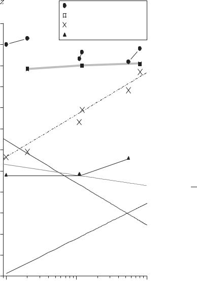
Fig. 6.7 A plot of the energy of various structures against atomic number Z. This includes the data shown on Fig. 6.5, but the scale has been changed to show the e ects of lower energy. The contributions to the isotope shift from the mass and volume e ects are plotted using eqns 6.21 and 6.26, respectively. Although these e ects arise from completely independent physical e ects, they have a similar magnitude for medium-heavy elements (and can be comparable to the magnetic dipole hyperfine structure of an excited state, which is considerably smaller than the ground-state splitting). The Doppler width for a visible transition with energy 2 eV is plotted to indicate the typical experimental limit in spectroscopic measurements using light; the

line has a slope of −1/2 because ∆f

√ D

1/ M and the atomic mass A is approximately A 2Z, so that ∆fD Z−1/2 (see eqn 8.7). For hydrogen the Doppler width is almost equal to the fine-structure splitting (and much larger than hyperfine structure). The Doppler broadening of visible lines in sodium is comparable with its hyperfine structure; for heavier elements the ground-state hyperfine structure can be resolved in a vapour at room temperature. This gives an indication of the importance of Doppler-free techniques described in Chapter 8. The Zeeman e ect of a magnetic flux density of B = 1 T is equivalent to a frequency shift of 14 GHz.

108 Hyperfine structure and isotope shift

22More accurate calculations can be made directly from eqn 6.24 in individual cases, e.g. the 1s configuration in

hydrogen has
4			r2						10−9 eV.
EVol =			N		hcR		5
			a02			∞		×
3

The proton has a root-mean-square charge radius of rN2 1/2 = 0.875 fm (CODATA value).

23The size of the nucleus rN2 generally increases with A following the trend in eqn 6.25 but there are exceptions, e.g. a nucleus that is particularly stable because it has closed shells of nucleons can be smaller than a lighter nucleus. Experimental measurements of isotope shifts, and the deduced values of the volume e ect, are used to study such behaviour. (Similarly, for atoms, the shell structure makes inert gas atoms exceptionally small. More generally, the variation of atomic size with atomic mass is opposite to that of ionization energy—alkali atoms are larger than nearby atoms in the periodic table.)

24See Woodgate (1980) for further details.

25High-energy electron scattering experiments also probe the nuclear charge distribution.

of a nucleus as
rN 1.2 × A1/3 fm .	(6.25)

Using this equation and making the same approximations for the wavefunction squared as in hyperfine structure (eqn 6.17), we can write the isotope shift caused by the volume e ect as

	∆E		r2			δA		Z2
%	Vol		N
		a02						(n )3 R∞ .		(6.26)
∆νVol = hc						A

This has been used to plot ∆EVol as a function of Z in Fig. 6.7, assuming that δA = 1, A 2Z and n 2.22

This volume e ect decreases the binding energy of a given atomic level with respect to that of a ‘theoretical’ atom with a point charge. The resulting change in the transition depends on whether the e ect occurs in the upper or lower level (see Exercise 6.9).23

6.2.3Nuclear information from atoms

We have shown that the nucleus has an observable e ect on atomic spectra. If hyperfine structure is observed then one immediately knows that the nucleus has spin and the number of hyperfine components sets a lower limit on I (Example 6.1). The values of F , and hence I, can be deduced by checking the interval rule, and the sum rule for relative intensities (similar to that for fine structure in Section 4.6.1). In principle, the magnetic moment of the nucleus µI can be deduced from the hyperfinestructure constant A, e.g. calculations such as that in Section 6.1.1 are accurate for light atoms. For atoms with a higher Z, the relativistic effects are important for the electronic wavefunction near the nucleus and it is more di cult to calculate |ψ (0)|2. However, the electronic factors cancel in ratios of the hyperfine-structure constants of isotopes of the same element to give accurate ratios of their magnetic moments, i.e. if the µI is known for one isotope then it can be deduced for the other isotopes (see Exercise 6.4).

Similarly, isotope shifts give the di erence in the nuclear sizes between

isotopes, ∆ rN2 , assuming that the mass e ects are calculable.24 To interpret this information, it is necessary to know the absolute value of the charge radius for one of the isotopes by another means, e.g. muonic

X-rays. These transitions between the energy levels of a muon bound to

an atomic nucleus have a very large volume e ect, from which rN2 can be deduced (see Exercise 6.13).25

6.3Zeeman e ect and hyperfine structure

The treatment of the Zeeman e ect on hyperfine structure (in the IJ- coupling scheme) closely resembles that described in Section 5.5 for the LS-coupling scheme, and the detailed explanation of each step is not repeated here. The total atomic magnetic moment of the atom is the

6.3 Zeeman e ect and hyperfine structure 109

sum of the electronic and nuclear moments (cf. eqn 5.9):

µatom = −gJ µBJ + gI µN I −gJ µBJ .

(6.27)

Since µN µB we can neglect the nuclear contribution (for all but the most precise measurements), so that the Hamiltonian for the interaction with an external field B is just that for the electronic magnetic moment:

H = gJ µBJ · B .

(6.28)

This interaction does not depend on the nuclear spin. However, its expectation value does depend on the hyperfine structure. We consider first the weak-field regime where the interaction with the external field is weaker than A I · J so that it can be treated as a perturbation to the hyperfine structure. We then treat the strong-field regime, and also the intermediate situation.

6.3.1Zeeman e ect of a weak field, µBB < A

If the interaction with the external field in eqn 6.28 is weaker than the hyperfine interaction A I · J, then in the vector model J and I move rapidly about their resultant F, as illustrated in Fig. 6.8, whilst F itself precesses more slowly about the magnetic field (z-axis). In this regime F and MF are good quantum numbers, but MI and MJ are not. Taking the projection of the magnetic moments along F gives the e ective Hamiltonian

H = g

µ

J · F

F

·

B = g

µ F

·

B = g

µ B F ,

(6.29)

B F (F + 1)

J

F

B

F

B

z

where

F (F + 1) + J (J + 1)

− I (I + 1)

gF =

gJ .

(6.30)

2F (F + 1)

Here the factor gF arises from the projection of J onto F, as illustrated in Fig. 6.9, in the just same way as gJ is given by the projection of L and S onto J in Section 5.5. The Zeeman energy is

E = gF µBBMF .

(6.31)

As an example, consider the ground-state hyperfine levels in hydrogen (I = J = 1/2 and gJ = gs 2 ). For F = 1 we find gF = 1 so the three states MF = −1, 0 and 1 are spaced by µBB. The F = 0, MF = 0 state has no first-order Zeeman shift (see Fig. 6.10).

In summary, the calculation of the Zeeman e ect of a weak magnetic field on the hyperfine structure is simple because only the magnetic moment of the electron(s) along J contributes, whereas in the LS-coupling scheme there are components along both L and S. However, I a ects gF because the nuclear angular momentum I is not small, and has a major e ect on the IJF -triangle (thinking in terms of vectors as in Fig. 6.9), even though the nuclear magnetic moment is negligible.

J

F

I

Fig. 6.8 The IJ-coupling scheme.

110 Hyperfine structure and isotope shift

Fig. 6.9 The projection of the contributions to the magnetic moment from the atomic electrons along F. The magnetic moment of the nucleus is negligible in comparison.

Fig. 6.10 The Zeeman e ect on the

1

0

hyperfine structure of the ground level

of hydrogen 1s

2S

. The interval be-

1/2

tween the F = 0 and F

=

1 levels

is A, as shown in Fig. 6.3.

The zero

1

2

of the energy scale has been chosen to

be midway between the levels at zero

field, which is

convenient

for the cal-

−1

culations in the text. (The two states

with MF = 0 in the low-field regime

are mixed by the perturbation and then

0

move apart as the magnetic flux density

increases.) The quantity x = µBB/A is

plotted on the horizontal axis and the

lowand high-field regimes correspond

Low field

High field

to x 1 and x

1.

26But smaller than the fine structure of the first excited state, except for the lightest elements. High-lying levels, however, have smaller fine structure.

6.3.2Zeeman e ect of a strong field, µBB > A

A strong field is one where the interaction with the external field, in eqn 6.28, is greater than A I · J. This can readily be achieved for hyperfine structures since the Zeeman energy µBB in a field of 1 T is about 6 × 10−5 eV (corresponding to a frequency of 14 GHz), which is greater than all but the largest hyperfine structures in the ground configurations of heavy elements (see Fig. 6.7).26 In this regime F is not a

6.3 Zeeman e ect and hyperfine structure 111

good quantum number and J precesses about B.27 The e ect of the hyperfine interaction can be calculated as a perturbation on the |IMI JMJ eigenstates, i.e.

EZE = gJ µBBMJ + IMI JMJ | A I · J |IMI JMJ	(6.32)
= gJ µBB MJ + A MI MJ .	(6.33)

The first term is the same as eqn 5.11. In the second term, I · J = IxJx + Iy Jy + Iz Jz and the x- and y-components average to zero in the precession about the field along the z-direction.28

An example of the energy levels in a strong field is shown in Fig. 6.10 for the hydrogen ground state. The two energy levels with MJ = ±1/2 are both split into sub-levels with MI = ±1/2 by the hyperfine interaction; eqn 6.33 shows that these sub-levels have a separation of A/2 (independent of the field strength).

6.3.3Intermediate field strength

In Fig. 6.10 the lowand high-field energy levels follow the rule that two states never cross if they have the same value of M , where at low fields M = MF and at high fields M = MI + MJ . This implies that

			MJ MI
F = 1,	MF = 0	→	+1/2, −1/2,
F = 0,	MF = 0	→	−1/2, +1/2.

This rule can be justified by showing that the operator Iz + Jz commutes with all the interactions and it allows unambiguous connection of states even in more complex cases.29 For the simple case of hydrogen the energy levels can be calculated at all fields by simple perturbation theory, as shown below.

Example 6.3 The Zeeman e ect on the hyperfine structure of hydrogen for all field strengths

Figure 6.10 shows the energy levels for all field strengths. The Zeeman energies of the M = ±1 states are ±µBB for all fields because their wavefunctions are not mixed (gF = 1 from eqn 6.30). The MF = 0 states have no first-order shift but the magnetic field mixes these two states in the F = 0 and 1 hyperfine levels; the matrix element between them is

− F = 1, MF = 0| µ · B |F = 0, MF = 0 = ζµBB .

Such (o -diagonal) matrix elements can be evaluated by angular momentum theory, but in this simple case we can get by without using Clebsch– Gordan coe cients (leaving ζ as an undetermined constant for the time being). The Hamiltonian for the two-level system is

	H =	A/2 ζµBB		.	(6.34)
		ζµBB	−A/2

27The nuclear angular momentum I does not precess around B because −µI ·B is negligible. In this regime the interaction A I·J makes I precess about the mean direction of J, which is parallel to B. Thus e ectively I precesses about the axis defined by B (but not because of −µI · B). The vector model picture requires careful thought because of the subtle di erences from the Paschen–Back e ect (Fig. 5.14). In the quantum mechanical description this is taken into account by considering the relative magnitudes of the pertur-

bations: |µe · B| > |A I · J| > |µI · B|, where µe is the magnetic moment of

the atomic electrons in eqn 5.9.

28This can be shown rigorously using the ladder operators

I+ ≡ Ix + i Iy ,

I− ≡ Ix − i Iy ,

and similarly for J+ and J−. These ladder operators change the magnetic quantum numbers, e.g.

I+ |I MI |I MI + 1 .

Since

IxJx + Iy Jy = 1 (I+J− + I−J+) ,

2

the expectation value of this part of I·J is zero (for states of given MJ and MI as in eqn 6.32).

29At low fields, Iz + Jz ≡ Fz , which clearly commutes with the interaction in eqn 6.29. At high fields the relevant interactions are proportional to Jz and IxJx + Iy Jy + Iz Jz , both of which commute with Iz + Jz .

112 Hyperfine structure and isotope shift

30Any choice for the point at which E = 0 leads to the same result, e.g. taking the unperturbed energies as A/4 and −3A/4 as in Fig. 6.3.

The energies are measured from the point midway between the hyperfine levels to streamline the algebra.30 The energy eigenvalues are

0

E = ± (A/2)2 + (ζµBB)2 . (6.35)

This exact solution for all fields is plotted in Fig. 6.10. The approximate solution for weak fields is

Eweak ±	A	+	(ζµBB)2	.	(6.36)
	2		A

31The avoided crossing of states that mix is a general feature of perturbation theory.

When B = 0 the two unperturbed levels have energies ±A/2. The term proportional to B2 is the usual second-order perturbation theory expression that causes the levels to avoid one another (hence the rule that states of the same M do not cross).31

For strong fields, where µBB A, eqn 6.35 gives the energy of the M = 0 states as

E(F = ±1, MF = 0) ±ζµBB .

(6.37)

In a strong field the energy levels of the system are given by gJ µBB MJ and the two MJ = ±1/2 states have Zeeman energies of gµBBMJ =

±µBB. Comparison with eqn 6.37 shows that ζ = 1, and so we have found the energies for all field strengths. The other two states have energies E(M = ±1) = 12 A ± µBB for all values of B.

A similar approach can be used when J = 1/2 for arbitrary values of I, which applies to the ground states of the alkalis. For I > 1/2 there are more states to consider than in hydrogen (where I = 1/2), so the Hamiltonian will have larger dimensions than in eqn 6.34. Actually there were four basis states to consider in hydrogen, but because the perturbation mixes only two of them it was only necessary to diagonalise a 2 × 2 matrix.

32The two spins are aligned in a triplet state so the 5sand 6s-electrons produce fields in the same direction.

6.4Measurement of hyperfine structure

An apparatus similar to that for measuring the Zeeman e ect, shown in Fig. 1.7(a), can be used to observe hyperfine structure—a magnet is not required because hyperfine structure arises from an internal magnetic field of the atom. Figure 6.11 shows a typical experimental trace obtained from such an experiment with a pressure-scanned Fabry–Perot ´etalon for the 5s5p 3P0−5s6s 3S1 line in cadmium. The 3P0 level has no hyperfine structure (because J = 0) and the observed splitting comes entirely from the 5s6s 3S1 level. Both s-electrons contribute to the field at the nucleus32 so this level has an exceptionally large hyperfine splitting that is greater than the Doppler broadening.

The fact that the J = 1 level only gives two hyperfine levels implies that I = 1/2. If I 1 then there would be three levels (by the rules for addition of angular momenta). One of these peaks might, however, be hidden underneath the large central peak? That this is not the case here

6.4 Measurement of hyperfine structure 113

(a)

Even isotopes (no HFS)

Lines

Fig. 6.11 (a) The 5s6s 3S1 level in the

from

odd isotopes of cadmium (111Cd and

(b)

even

113Cd) has a large hyperfine structure;

isotopes

the

F

=

3/2 hyperfine level lies be-

Transmitted

low

F

=

1/2 because the nuclear g-

intensity

factor

is

negative and similar in size

for both odd isotopes. (The total mag-

netic field created by the unpaired s-

electrons at the nucleus is anti-parallel

to J, as in the ground state of hydro-

gen

and

the alkalis.)

(b) An exper-

imental trace of the hyperfine struc-

ture

for

the 5s5p 3P0–5s6s 3S1 line

at a

wavelength of

468 nm obtained

with a pressure-scanned Fabry–Perot

´etalon (as in Fig. 1.7). There are three

peaks in each order of the ´etalon: a

large peak from the isotopes with no

nuclear spin I = 0 and hence no hyper-

fine structure (generally isotopes with

an even number of nucleons so there are

no unpaired spins within the nucleus);

and two smaller peaks whose separa-

tion equals the hyperfine splitting of

Frequency (GHz)

the 5s6s 3S1 level. (Data from the Ox-

0

10

20

30

ford Physics Teaching Laboratory prac-

tical course; further details are in Lewis (1977).)

can be checked by verifying that the observed peaks have the expected displacements from their centre of gravity (which is approximately at the position of the even isotopes).33

It can be seen from Fig. 6.11 that optical spectroscopy is not generally suitable for measuring the Zeeman e ect of hyperfine structure because spectral lines have a Doppler broadening that can be comparable with the hyperfine splitting. Thus in the low-field regime (µBB < A) the Zeeman splitting is too small to be resolved. To show this quantitatively

33This is not straightforward in this example because of the overlap of lines, but this could be done using a curvefitting program on a computer. Additionally, there is a sum rule for the intensities as in fine structure.

114 Hyperfine structure and isotope shift

we consider the Doppler width ∆fD of a line of wavelength λ:

∆fD	2u	,	(6.38)
	λ

34This gives a value of ∆fD that di ers

√

by only ln 2 = 0.8 from the exact result for the full width at half maximum (FWHM) derived in Chapter 8.

35The Zeeman splitting of a spectral line can only be resolved when the field is strong enough to give the Paschen– Back e ect.

where u is a typical atomic velocity. The factor of 2 appears because

atoms can move towards and away from the observer. For this estimate

we shall use the most probable velocity u = 2kBT /m.34 For cadmium at T = 300 K, we have u 200 m s−1 and thus the Doppler width of the lines with a wavelength of λ = 468 nm is ∆fD = 2u/λ = 0.9 GHz, whereas A = 7.9 GHz for the 5s6s 3S1 level. More generally, the Doppler width for a visible transition is plotted in Fig. 6.7 as a function of the atomic number. At room temperature the optical transitions of hydrogen, the lightest element, have a Doppler width slightly less than the fine-structure splitting of the first excited state, so in this case the lowfield Zeeman e ect cannot be observed even for fine structure (let alone hyperfine structure).35 Figure 6.12 shows the results of an experimental observation of the hyperfine structure and isotope shift of tin by a technique of Doppler-free laser spectroscopy (that will be described in Section 8.2).

Doppler broadening is much less of a problem in direct measurements of the separation between hyperfine levels with microwave techniques (at frequencies of gigahertz), or the even smaller splitting of the Zeeman sub-levels that correspond to radio-frequency transitions. An example of a radio-frequency and microwave spectroscopy technique is outlined in the next section.

Fig. 6.12 Doppler-free laser spectroscopy of the 5p2 3P0–5p6s 3P1 line of tin; the reduction in Doppler broadening (cf. Fig. 6.11) reveals the isotope shifts between the even isotopes, in addition to the hyperfine splitting of the odd isotopes. Each peak is labelled by the relative atomic mass. Each odd isotope gives rise to two peaks because of hyperfine structure (as in Fig. 6.11). For further details see Baird et al. (1983).

6.4.1The atomic-beam technique

An atomic-beam apparatus can be understood as an extension of the original Stern–Gerlach apparatus illustrated in Fig. 6.13. In the original Stern–Gerlach experiment a beam of silver atoms was sent through a region of strong gradient of the magnetic field and further downstream the atoms were deposited on a glass plate. Upon inspecting the plate, Stern and Gerlach found that the atoms appeared in two distinct places, showing that the atomic beam was split into two directions. This told them that angular momentum is quantised and that it can have values

			120
			118
			116
117a 119a	112	114	122	124	117b	119b

Frequency

6.4 Measurement of hyperfine structure 115

Beam source

Collimator

Magnet

Atoms deposited in two places

that are half-integer multiples of . (Orbital angular momentum would give 2l + 1 components, with l an integer.) To interpret the experiment we consider an atom in a magnetic field B with a gradient along the z-axis.36 The force exerted on the atom is (using eqn 5.11)

Force = −	dEZE	= gJ µB	dB	MJ .	(6.39)
	dz		dz

The ground level of silver, 5s 2S1/2, has l = 0 and J = s = 1/2. Thus the force on atoms passing through the Stern–Gerlach magnet has the two values F = ±µB dB/dz for ms = MJ = ±21 . This explains the separation of the atomic beam into two components and provides direct observational evidence for quantisation since the two emerging beams are well defined. For a classical vector the z-component of angular momentum would be spread over a range between the maximum and minimum values.

An atomic-beam apparatus has two Stern–Gerlach-type magnets, as shown in Fig. 6.14, that create an inhomogeneous field in the A and B regions to deflect atoms according to their MJ state. The A and B regions have a strong field (µBB A), associated with the high gradient of magnetic field there, so MJ is a good quantum number and eqn 6.39 gives the force. The transition to be measured occurs in the C region between the two state-selecting magnets where, generally, the atoms are in the low-field regime. The principles of the operation of such an

Fig. 6.13 In the original Stern–Gerlach apparatus a beam of silver atoms was sent through a region of strong gradient of the magnetic field and further downstream the atoms were deposited on a glass plate. This simple experiment had a great influence on the development of quantum ideas and provides a very useful illustration of the concepts of quantisation (Feynman et al. 1963– 1965).

36Since · B = 0 we cannot have a gradient along the z-axis without there also being a gradient in another direction, but the e ect of a gradient in a direction perpendicular to B averages to zero as the magnetic moment precesses around the z-axis—for a more rigorous discussion see Chapter 10.