Atomic physics (2005)

e2

K1snl = 4π 0

56 Helium

25At small r the wavefunction of an ns-electron deviates significantly from uZns=1; for this reason 1s2p was chosen as an example above.

26The overlap of the 1s and nl wavefunctions becomes smaller as n and l increase. In Heisenberg’s treatment where screening is taken into account, the direct integral gives the deviation from the hydrogenic levels (which could be characterised by a quantum defect as in the alkalis, see Chapter 4).

2	2			0 the term
For electrons with l			=
l (l + 1) /2mr		in	the	Schr¨odinger

equation causes the electron’s wave-

function to lie almost entirely outside the region where uZ1s=2 = R1s (r) /√4π has a significant value.

unlm = Rnl(r)Ylm (θ, φ) only the radial part depends on Z. We write the exchange integral as (cf. eqn 3.28)

K(r1, r2)R1s(r1)Rnl(r1)R1s(r2)Rnl(r2)r12 dr1 r22 dr2 .

(3.32) The function K(r1, r2) containing the angular integrals is (cf. eqn 3.29)

K(r1, r2) =	r12 Ylm		(θ1	, φ1) 4π Ylm(θ2, φ2)		(3.33)
	1			1

× sin θ1 dθ1 dφ1 sin θ2 dθ2 dφ2 .

For the 1snp configuration only the second term of the expansion in eqn 3.30, with k = 1, survives in the integration because of the orthogonality of the spherical harmonic functions (see Exercise 3.7), to give

	r1	/3r2	for r1	< r2	,
K(r1	, r2) =	2			(3.34)
		/3r2	for r
	r			< r .
	2	1	2	1

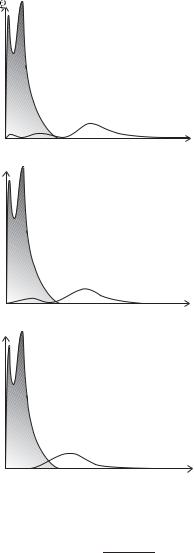
Carrying out the integration over the radial wavefunctions in eqn 3.32 for the 1s2p configuration gives the splitting between 3P and 1P as 2K1s2p 0.21 eV (close to the measured value of 0.25 eV).

The assumption that the excited electron lies outside the 1s wavefunction does not work so well for 1sns configurations since ψns (0) has a finite value and the above method of calculating J and K is less accurate.25 The 1s2s configuration of helium has a singlet–triplet sepa-

ration of E 1S			− E 3S	= 2K1s2s 0.80 eV and the direct integral is
	than that for 1s2p—these trends are evident in Fig. 3.4 (see
also larger			26
also Exercise 3.7).

In some respects, helium is a more typical atom than hydrogen. The Schr¨odinger and Dirac equations can be solved exactly for the oneelectron system, but not for helium or other atoms with more electrons. Thus in a careful study of helium we encounter the approximations needed to treat multi-electron atoms, and this is very important for understanding atomic structure in general. Helium also gives a good example of the influence of identical particles on the occupation of the states in quantum systems. The energy levels of the helium atom (and the existence of exchange integrals) do not depend on the fact that the two electrons are identical, as demonstrated in Exercises 3.3 and 3.4; however, this is a common point of confusion. The books recommended for further reading give clear and accurate descriptions of helium that reward careful study.

Further reading

The recommended books are divided into two categories corresponding to the two main themes in this chapter: (a) a description of how to calculate the electrostatic energy in an atom with more than one electron, which introduces principles that can be used in atoms with more

3.3 Evaluation of the integrals in helium 57

electrons; and (b) a discussion of the influence of identical particles on the statistics of a quantum system that is important throughout physics. The influence of identical particles on the occupation of the quantum levels of a system with many particles, i.e. Bose–Einstein and Fermi–Dirac statistics, is discussed in statistical mechanics texts. Clear descriptions of helium may be found in the following textbooks: Cohen-Tannoudji et al. (1977), Woodgate (1980) and Mandl (1992). The calculation of the direct and exchange integrals in Section 3.3 is based on the definitive work by Bethe and Salpeter (1957), or see Bethe and Jackiw (1986).

A very instructive comparison can be made between the properties of the two electrons in helium and the nuclear spin statistics of homonuclear diatomic molecules27 described in Atkins (1983, 1994).28 There are diatomic molecules with nuclei that are identical bosons, identical fermions and cases of two similar but not identical particles, and their study gives a wider perspective than the study of helium alone. The nuclei of the two atoms in a hydrogen molecule are protons which are fermions (like the two electrons in helium).29 For reasons explained in the above references, we can consider only those parts of the molecular wavefunction that describe the rotation ψrot and the nuclear spin states ψI —these are spatial and spin wavefunctions, respectively. For H2 the wavefunction must have overall antisymmetry with respect to an interchange of particle labels since the nuclei are protons, each with a spin of 1/2. This requires that a rotational must pair with a spin function of the opposite symmetry:

ψ	= ψS	ψA	or	ψA	ψS .	(3.35)
molecule	rot	I		rot	I

This is analogous to eqn 3.18 for helium; as described in Section 3.2.1, the two spin-1/2 nuclei in a hydrogen molecule give a total (nuclear) spin of 0 and 1, with one state and three states, respectively. The 1 to 3 ratio of the number of nuclear spins associated with the energy levels for ψrotS and ψrotA , respectively, influences the populations of these rotational energy levels in a way that is directly observed in molecular spectra (the intensity of the lines in spectra depends on the population of the initial level). The molecule HD made from hydrogen and deuterium does not have identical nuclei so there is no overall symmetry requirement, but it has similar energy levels to those of H2 apart from the mass dependence. This gives a real physical example where the statistics depends on whether the particles are identical or not, but the energy of the system does not. Exercise 3.4 discusses an artificial example: a helium-like system that has the same energy levels as a helium atom and hence the same direct and exchange integrals, even though the constituent particles are not identical.

27Molecules made up of two atoms with identical nuclei.

28These books also summarise the helium atom and the quantum mechanics of these molecular systems is very closely related to atomic physics.

29The wavefunction of the hydrogen molecule has exchange symmetry—

crudely speaking, the molecule looks the same when rotated through 180◦.

58 Helium

Exercises

More advanced problems are indicated by a *.

(3.1) Estimate of the binding energy of helium

(a)Write down the Schr¨odinger equation for the helium atom and state the physical significance of each of the terms.

(b)Estimate the equilibrium energy of an electron bound to a charge +Ze by minimising

	2		Ze2
E(r) =		−		.
	2mr2		4π 0r

(c)Calculate the repulsive energy between the two electrons in helium assuming that r12 r. Hence estimate the ionization energy of helium.

(d)Estimate the energy required to remove a further electron from the helium-like ion Si12+, taking into account the scaling with Z of the energy levels and the expectation value for the electrostatic repulsion. The experimen-

tal value is 2400 eV. Compare the accuracy of your estimates for Si12+ and helium. (IE(He) = 24.6 eV.)

(3.2) Direct and exchange integrals for an arbitrary system

(a) Verify that for

ψA(r1, r2)

1

= √

{uα(r1)uβ (r2) − uα(r2)uβ (r1) }

2

and

H

=

e2/4π 0r12 the expectation value

S

ψA

H

ψA

has the form J − K and give the

expressions for J and K.

(b)

Write down the wavefunction ψ that is orthog-

onal to ψA.

(c)

Verify that

ψA

H

ψS

= 0 so that H is di-

agonal in

this basis.

(3.3) Exchange integrals for a delta-function interaction

A particle in a square-well potential, with V (x) = 0 for 0 < x < and V (x) = ∞ elsewhere, has

normalised eigenfunctions u				(x) =	2/ sin (πx/ )
and u1	(x) = 2/ sin (2πx/0 ).

(a)What are the eigenenergies E0 and E1 of these two wavefunctions for a particle of mass m?

(b)Two particles of the same mass m are both in the ground state so that the energy of the whole system is 2E0. Calculate the perturbation produced by a point-like interaction described by the potential a δ (x1 − x2), with a constant.

(c)Show that, when the two interacting particles occupy the ground and first excited states, the direct and exchange integrals are equal. Also show that the delta-function interaction produces no energy shift for the antisymmetric spatial wavefunction and explain this in terms of correlation of the particles. Calculate the energy of the other level of the perturbed system.

(d)For the two energy levels found in part (c), sketch the spatial wavefunction as a function of the coordinates of the two particles x1 and x2. The particles move in one dimension but the two-particle wavefunction exists in a twodimensional Hilbert space—draw either a contour plot in the x1x2-plane or attempt a threedimensional sketch (by hand or computer).

(e)The two particles are identical and have spin 1/2. What is the total spin quantum number S associated with each of the energy levels found in part (c)?

(f) Discuss qualitatively the energy levels of this system for two particles that have slightly different masses m1 = m2, so that they are distinguishable? [Hint. The spin has not been given because it is not important for non-identical particles.]

Comment. The antisymmetric spatial wavefunction in part (c) clearly has di erent properties from a straightforward product u0u1. The exchange integral is a manifestation of the entanglement of the multiple-particle system.

(3.4) A helium-like system with non-identical particles

Imagine that there exists an exotic particle with the same mass and charge as the electron but spin 3/2 (so it is not identical to the electron). This particle and an electron form a bound system with a helium nucleus. Compare the energy levels of this system with those of the helium atom. Describe the energy levels of a system with two of the ex-

Exercises for Chapter 3 59

otic particles bound to a helium nucleus (and no

is

electrons). [Hint. It is not necessary to specify the

1 − 2

2 −1/2

values of total spin associated with the levels.]

1

1

r1

r1

=

cos θ12 +

(3.5)

The integrals in helium

r12

r2

r2

r2

(a)

Show that the integral in eqn 3.24 gives the

1

r1

1 +

cos θ12 + . . . .

(3.36)

value stated in eqn 3.7.

r2

r2

(b)

Estimate the ground-state energy of helium us-

(When r1 > r2 we must interchange r1 and r2 to ob-

ing the variational principle. (The details of

tain convergence.) The cosine of the angle between

this technique are not given in this book; see

r1 and r2 is

the section on further reading.)

(3.6)

Calculation of integrals for the 1s2p configuration

cos θ12 = r1 · r2

(a) Draw a

scale diagram of R1sZ=2 (r), R2sZ=1 (r)

−

= cos θ1 cos θ2 + sin θ1 sin θ2 cos (φ1

φ2) .

and R2pZ=1 (r). (See Table 2.2.)

(b)

Calculate the direct integral in eqn 3.31 and

(a)

Show that the first two terms in the binomial

expansion agree with the terms with k = 0 and

show that it gives

1 in eqn 3.30.

e2/4π 0

13

(b)

The repulsion between a 1sand an nl-electron

J1s2p = − 2a0

2 × 55 .

is independent of m. Explain why, physically

Give the numerical value in eV (cf. that given

or mathematically.

in the text).

(c)

Show that eqn 3.32 leads to eqn 3.34 for l = 1.

(3.7)

Expansion of 1/r12

(d)

For a 1snl configuration, the quantity K(r1, r2)

For r1 < r2 the binomial expansion of

in eqn 3.34 is proportional

l

l+1

when

to r1

/r2

1

2

2

1/2

r1 < r2.

Explain this in terms of mathemat-

= r1

+ r2 − 2r1r2 cos θ12

−

ical properties of the Yl,m functions.

r12

Web site:

http://www.physics.ox.ac.uk/users/foot

This site has answers to some of the exercises, corrections and other supplementary information.

4	The alkalis

4.1	Shell structure and the
	periodic table	60
4.2	The quantum defect	61
4.3	The central-field
	approximation	64
4.4	Numerical solution of the
	Schr¨odinger equation	68
4.5	The spin–orbit interaction:
	a quantum mechanical
	approach	71
4.6	Fine structure in the alkalis 73
Further reading		75
Exercises		76

1Also referred to by its original German name as the Aufbauprinciple. An extensive discussion of the atomic structure that underlies the periodic table can be found in chemistry texts such as Atkins (1994).

2Most of the arrangement of elements in a periodic table was determined by chemists, such as Mendeleev, in the nineteenth century. A few inconsistencies in the ordering were resolved by Moseley’s measurements of X-ray spectra (see Chapter 1).

3The configuration of an atom is specified by a list of nl with the occupancy as an exponent. Generally, we do not need to list the full configuration and it is su cient to say that a sodium atom in its ground state has the configuration 3s. A sodium ‘atom’ with one electron in the 3s level, and no others, is an excited state of the highly-charged ion Na+10—this esoteric system can be produced in the laboratory but confusion with the common sodium atom is unlikely.

4.1Shell structure and the periodic table

For multi-electron atoms we cannot solve the Hamiltonian analytically, but by making appropriate approximations we can explain their structure in a physically meaningful way. To do this, we start by considering the elementary ideas of atomic structure underlying the periodic table of the elements. In the ground states of atoms the electrons have the configuration that minimises the energy of the whole system. The electrons do not all fall down into the lowest orbital with n = 1 (the K-shell) because the Pauli exclusion principle restricts the number of electrons in a given (sub-)shell—two electrons cannot have the same set of quantum numbers. This leads to the ‘building-up’ principle: electrons fill up higher and higher shells as the atomic number Z increases across the periodic table.1 Full shells are found at atomic numbers Z = 2, 10, . . .

corresponding to helium and the other inert gases. These inert gases, in a column on the right-hand side of the periodic table (see inside front cover), were originally grouped together because of their similar chemical properties, i.e. the di culty in removing an electron from closed shells means that they do not readily undergo chemical reactions.2 However, inert gas atoms can be excited to higher-lying configurations by bombardment with electrons in a gas discharge, and such processes are very important in atomic and laser physics, as in the helium–neon laser.

The ground states of the alkalis have the following electronic configurations:3

lithium	Li	1s2	2s ,
sodium	Na	1s2	2s22p6	3s ,
potassium	K	1s2	2s22p6	3s23p6	4s ,
rubidium	Rb	1s2	2s22p6	3s23p6	3d10	4s24p6 5s ,
caesium	Cs	1s2	2s22p6	3s23p6	3d10	4s24p64d105s25p6 6s .

The alert reader will notice that the sub-shells of the heavier alkalis are not filled in the same order as the hydrogenic energy levels, e.g. electrons occupy the 4s level in potassium before the 3d level (for reasons that emerge later in this chapter). Thus, strictly speaking, we should say that the inert gases have full sub-shells, e.g. argon has the electronic

4.2 The quantum defect 61

Table 4.1 Ionization energies of the inert gases and alkalis.

Element	Z	IE (eV)
He	2	24.6
Li	3	5.4
Ne	10	21.6
Na	11	5.1
Ar	18	15.8

K19 4.3

Kr	36	14.0
Rb	37	4.2
Xe	54	12.1
Cs	55	3.9

configuration 1s22s22p63s23p6 with the 3d sub-shell unoccupied.4

Each alkali metal comes next to an inert gas in the periodic table and much of the chemistry of the alkalis can be explained by the simple picture of their atoms as having a single unpaired electron outside a core of closed electronic sub-shells surrounding the nucleus. The unpaired valence electron determines the chemical bonding properties; since it takes less energy to remove this outer electron than to pull an electron out of a closed sub-shell (see Table 4.1), thus the alkalis can form singlycharged positive ions and are chemically reactive.5 However, we need more than this simple picture to explain the details of the spectra of the alkalis and in the following we shall consider the wavefunctions.

4.2The quantum defect

The energy of an electron in the potential proportional to 1/r depends only on its principal quantum number n, e.g. in hydrogen the 3s, 3p and 3d configurations all have the same gross energy. These three levels are not degenerate in sodium, or any atom with more than one electron, and this section explains why. Figure 4.1 shows the probability density of 3s-, 3pand 3d-electrons in sodium. The wavefunctions in sodium have a similar shape (number of nodes) to those in hydrogen. The 3d wavefunction has a single lobe outside the core so that it experiences almost the same potential as in a hydrogen atom; therefore this electron, and other d configurations in sodium with n > 3, have binding energies similar to those in hydrogen, as shown in Fig. 4.2. In contrast, the wavefunctions for the s-electrons have a significant value at small r— they penetrate inside the core and ‘see’ more of the nuclear charge. Thus the screening of the nuclear charge by the other electrons in the atom is less e ective for ns configurations than for nd, and s-electrons have lower energy than d-electrons with the same principal quantum number. (The np-electrons lie between these two.6) The following modified form of

4This book takes a shell to be all energy levels of the same principal quantum number n, but the meaning of shell and sub-shell may be di erent elsewhere. We use sub-shell to denote all energy levels with specific values of n and l (in a shell with a given value of n). We used these definitions in Chapter 1; the inner atomic electrons involved in X-ray transitions follow the hydrogenic ordering.

5For a plot of the ionization energies of all the elements see Grant and Phillips (2001, Chapter 11, Fig. 18). This figure is accessible at http://www. oup.co.uk/best.textbooks/physics/ ephys/illustrations/.

6This dependence of the energy on the quantum number l can also be explained in terms of the elliptical orbits of Bohr–Sommerfeld quantum theory rather than Schr¨odinger’s wavefunctions; however, we shall use only the ‘proper’ wavefunction description since the detailed correspondence between the elliptical classical trajectories and the radial wavefunctions can lead to confusion.

62 The alkalis

(a)

Core

Fig. 4.1 The probability density of the electrons in a sodium atom as a function of r. The electrons in the n = 1 and n = 2 shells make up the core, and the probability density of the unpaired outer electron is shown for the n = 3 shell with l = 0, 1 and 2. The probability is proportional to |P (r)|2 = r2|R(r)|2; the r2 factor accounts for the increase in volume of the spherical shell between r and r + dr (i.e. 4πr2 dr) as the radial distance increases. The decreasing penetration of the core as l increases can be seen clearly—the 3delectron lies mostly outside the core with a wavefunction and binding energy very similar to those for the 3d configuration in hydrogen. These wavefunctions could be calculated by the simple numerical method described in Exercise 4.10, making the ‘frozen core’ approximation, i.e. that the distribution of the electrons in the core is not a ected by the outer electron—this gives su cient accuracy to illustrate the qualitative features. (The iterative method described in Section 4.4 could be used to obtain more accurate numerical wavefunctions.)

0

(b)

Core

0

(c)

Core

0

Bohr’s formula works amazingly well for the energy levels of the alkalis:

R∞

E (n, l) = −hc . (4.1) (n − δl)2

7This di ers from the modification used for X-ray transitions in Chapter 1—hardly surprising since the physical situation is completely di erent for the inner and outer electrons.

A quantity δl, called the quantum defect, is subtracted from the principal quantum number to give an e ective principal quantum number n = n − δl.7 The values of the quantum defects for each l can be estimated by inspecting the energy levels shown in Fig. 4.2. The d-electrons have a very small quantum defect, δd 0, since their energies are nearly hydrogenic. We can see that the 3p configuration in sodium has comparable energy to the n = 2 shell in hydrogen, and similarly for 4p and n = 3, etc.; thus δp 1. It is also clear that the quantum defect for s-electrons is greater than that for p-electrons. A more detailed analysis shows that all the energy levels of sodium can be parametrised by the above formula and only three quantum defects:

4.2 The quantum defect 63

−
−
−
−
−
−
δs = 1.35 ,	δp = 0.86 ,	δd = 0.01 ,	δl 0.00	for	l > 2 .

There is a small variation with n (see Exercise 4.3). Having examined the variation in the quantum defects with orbital angular momentum quantum number for a given element, now let us compare the quantum defects in di erent alkalis. The data in Table 4.1 show that the alkalis have similar ionization energies despite the variation in atomic number. Thus the e ective principal quantum numbers n = (13.6 eV/IE)1/2

Fig. 4.2 The energies of the s, p, d and f configurations in sodium. The energy levels of hydrogen are marked on the right for comparison. The guidelines link configurations with the same n to show how the energies become closer to the hydrogenic values as l increases, i.e. the quantum defects decrease so that δl 0 for f-electrons (and for the configurations with l > 3 that have not been drawn).

64 The alkalis

Table 4.2 The e ective principal quantum numbers and quantum defects for the ground configuration of the alkalis. Note that the quantum defects do depend slightly on n (see Exercise 4.3), so the value given in this table for the 3s-electron in sodium di ers slightly from the value given in the text (δs = 1.35) that applies for n > 5.

Element	Configuration	n	δs
Li	2s	1.59	0.41
Na	3s	1.63	1.37
K	4s	1.77	2.23
Rb	5s	1.81	3.19
Cs	6s	1.87	4.13

8For example, lithium has three interactions between the three electrons, inversely proportional to r12, r13 and r23; summing over all j for each value of i would give six terms.

(from eqn 4.1) are remarkably similar for all the ground configurations of the alkalis, as shown in Table 4.2.

In potassium the lowering of the energy for the s-electrons leads to the 4s sub-shell filling before 3d. By caesium (spelt cesium in the US) the 6s configuration has lower energy than 4f (δf 0 for Cs). The exercises give other examples, and quantum defects are tabulated in Kuhn (1969) and Woodgate (1980), amongst others.

4.3The central-field approximation

The previous section showed that the modification of Bohr’s formula by the quantum defects gives reasonably accurate values for the energies of the levels in alkalis. We described an alkali metal atom as a single electron orbiting around a core with a net charge of +1e, i.e. the nucleus surrounded by N − 1 electrons. This is a top-down approach where we consider just the energy required to remove the valence electron from the rest of the atom; this binding energy is equivalent to the ionization energy of the atom. In this section we start from the bottom up and consider the energy of all the electrons. The Hamiltonian for N electrons in the Coulomb potential of a charge +Ze is

N		2		2	Ze2/4π 0	N	e2/4π 0	.
H =				i		+			(4.2)
				−	ri	j>i	rij
i=1 −2m

The first two terms are the kinetic energy and potential energy for each electron in the Coulomb field of a nucleus of charge Z. The term with rij = |ri − rj | in the denominator is the electrostatic repulsion between the two electrons at ri and rj . The sum is taken over all electrons with j > i to avoid double counting.8 This electrostatic repulsion is too large to be treated as a perturbation; indeed, at large distances the repulsion cancels out most of the attraction to the nucleus. To proceed further we make the physically reasonable assumption that a large part of the repulsion between the electrons can be treated as a central potential

4.3 The central-field approximation 65

S (r). This follows because the closed sub-shells within the core have a spherical charge distribution, and therefore the interactions between the di erent shells and between shells and the valence electron are also spherically symmetric. In this central-field approximation the total potential energy depends only on the radial coordinate:

VCF (r) = −	Ze2/4π 0			+ S(r) .	(4.3)
			r
In this approximation the Hamiltonian becomes
N
		2
HCF = i=1 −			i2 + VCF (ri) .		(4.4)
		2m

For this form of potential, the Schr¨odinger equation for N electrons, Hψ = Eatomψ, can be separated into N one-electron equations, i.e. writing the total wavefunction as a product of single-electron wavefunctions, namely

	ψatom = ψ1ψ2ψ3 · · · ψN ,		(4.5)
leads to N equations of the form
−	2
		12 + VCF (r1) ψ1 = E1ψ1 ,	(4.6)
	2m

and similar for electrons i = 2 to N . This assumes that all the electrons see the same potential, which is not as obvious as it may appear. This symmetric wavefunction is useful to start with (cf. the treatment of helium before including the e ects of exchange symmetry); however, we know that the overall wavefunction for electrons, including spin, should be antisymmetric with respect to an interchange of the particle labels. (Proper antisymmetric wavefunctions are used in the Hartree– Fock method mentioned later in this chapter.) The total energy of the system is Eatom = E1 + E2 + . . . + EN . The Schr¨odinger equations for each electron (eqn 4.6) can be separated into parts to give wavefunctions of the form ψ1 = R(r1)Yl1 ,m1 ψspin(1). Angular momentum is conserved in a central field and the angular equation gives the standard orbital angular momentum wavefunctions, as in hydrogen. In the radial equation, however, we have VCF(r) rather than a potential proportional to 1/r and so the equation for P (r) = rR (r) is

−	2 d2				2l (l + 1)	P (r) = EP (r) . (4.7)
				+ VCF (r) +
	2m		dr2		2mr2

To solve this equation we need to know the form of VCF(r) and compute the wavefunctions numerically. However, we can learn a lot about the behaviour of the system by thinking about the form of the solutions, without actually getting bogged down in the technicalities of solving the equations. At small distances the electrons experience the full nuclear charge so that the central electric field is

E(r) →	Ze	r .	(4.8)
	4π 0r2