Atomic physics (2005)

46 Helium

2 √

1/ 4π is the angular part of an s- electron wavefunction.

3This is a standard quantum mechanical technique whose mathematical details are given in quantum texts. The essential principle of this technique is to find an expression for the energy in terms of a parameter—an e ective atomic number in the case of helium— and then minimise the energy with respect to this parameter, i.e. study the variation in the energy as a function of the chosen parameter.

4This is accessible at http://www. oup.co.uk/best.textbooks/physics/ ephys/illustrations/ along with other illustrations of elementary quantum ideas.

5It is often said that ‘one electron is in a spin-up state and the other is spindown’; what this really means is defined in the discussion of spin for the excited states of helium.

Now we need to calculate the perturbation produced by the electron– electron repulsion. The system has the spatial wavefunction

ψ1s2 = R1sZ=2 (r1) R1sZ=2 (r2) ×	1	,	(3.6)
	4π

where radial wavefunctions are defined in Table 2.2.2 The expectation value of the repulsion is (see Section 3.3)

e2		∞ ∞		1
	0	0	ψ1s	2		ψ1s2	r12 dr1 r22 dr2	= 34 eV .	(3.7)
4π 0					r12

Adding this to the (zeroth-order) estimate E(0) gives an energy of E(1s2) = −109 + 34 = −75 eV. It takes an energy of 75 eV to remove both electrons from a helium atom leaving a bare helium nucleus He++— the second ionization energy. To go from He+ to He++ takes 54.4 eV, so this estimate suggests that the first ionization energy (required to remove one electron from He to create He+) is IE(He) 75 − 54 21 eV. But the expectation value in eqn 3.7 is not small compared to the binding energy and therefore the perturbation has a significant e ect on the wavefunctions. The necessary adjustment of the wavefunctions can be accounted for by the variational method.3 This method gives a value close to the measured ionization energy 24.6 eV. Helium has the highest first ionization energy of all elements because of its closed n = 1 shell. For a plot of the ionization energies of the elements see Grant and Phillips (2001, Chapter 11, Fig. 18).4

According to the Pauli exclusion principle, two electrons cannot have the same set of quantum numbers. Therefore there must be some additional quantum number associated with the two 1s-electrons in the ground state of helium—this is their spin (introduced in Section 2.3.1). The observed filling-up of the atomic (sub-)shells in the periodic table implies that two spin states are associated with each set of spatial quantum numbers n, l, ml.5 However, electrostatic energies do not depend on spin and we can find the spatial wavefunctions separately from the problem of finding the spin eigenfunctions.

6The spatial wavefunction u contains both radial and angular parts but the energy does not depend on the magnetic quantum number, so we drop m as a subscript on u. The repulsion from a spherically-symmetric 1s wavefunction does not depend on the orientation of the other electron. To show this mathematically we could carry m through all the calculations and examine the resulting angular integrals, but this is cumbersome.

3.2Excited states of helium

To find the energy of the excited states we use the same procedure as for the ground state—at first we neglect the mutual repulsion term and separate eqn 3.1 into two one-electron equations that have solutions6

1
u1s(1) = R1s(r1) ×	√		,
		4π

unl(2) = Rnl(r2)Yl,m (θ2, φ2)

for the configuration 1snl. The spatial part of the atomic wavefunction is the product

ψspace = u1s(1)unl(2) .

(3.8)

Another wavefunction has the same energy, namely
ψspace = u1s(2)unl(1) .	(3.9)

These two states are related by a permutation of the labels on the electrons, 1 ↔ 2; the energy cannot depend on the labeling of identical particles so there is exchange degeneracy. To consider the e ect of the repulsive term on this pair of wavefunctions with the same energy (degenerate states) we need degenerate perturbation theory. There are two approaches. The look-before-you-leap approach is first to form eigenstates of the perturbation from linear combinations of the initial states.7 In this new basis the determination of the eigenenergies of the states is simple. It is instructive, however, simply to press ahead and go through the algebra once.8

We rewrite the Schr¨odinger equation (eqn 3.1) as
(H0 + H ) ψ = Eψ ,	(3.10)

where H0 = H1 + H2, and we consider the mutual repulsion of the electrons H = e2/4π 0r12 as a perturbation. We also rewrite eqn 3.2 as

H0ψ = E(0)ψ ,

(3.11)

where E(0) = E1 + E2 is the unperturbed energy. Subtraction of eqn 3.11 from eqn 3.10 gives the energy change produced by the perturbation, ∆E = E − E(0), as

H ψ = ∆E ψ .

(3.12)

A general expression for the wavefunction with energy E(0) is a linear combination of expressions 3.8 and 3.9, with arbitrary constants a and b,

ψ = a u1s(1)unl(2) + b u1s(2)unl(1) .	(3.13)
Substitution into eqn 3.12, multiplication by either	u1s(1)unl(2) or

u1s(2)unl(1), and then integration over the spatial coordinates for each electron (r1, θ1, φ1 and r2, θ2, φ2) gives two coupled equations that we

write as		J	K		a			a
	K		J		b	= ∆E b .			(3.14)
This is eqn 3.12 in matrix form. The direct integral is
J =	1		|u1s(1)|2			e2	|unl(2)|2 dr13 dr23
	4π 0					r12
	1			ρ1s(r1)ρnl(r2)
=								dr13 dr23 ,	(3.15)
	4π 0				r12
where ρ1s(1) = −e |u1s(1)|2			is the charge density distribution for elec-

tron 1, and similarly for ρnl(2). This direct integral represents the Coulomb repulsion of these charge clouds (Fig. 3.1). The exchange integral is

K =	1		u1s(1)unl	(2)	e2	u1s(2)unl(1) dr13 dr23 .	(3.16)
	4π 0				r12

3.2 Excited states of helium 47

7This is guided by looking for eigenstates of symmetry operators that commute with the Hamiltonian for the interaction, as in Section 4.5.

8In the light of this experience one can take the short cut in future.

48 Helium

Fig. 3.1 The direct integral in a 1sns configuration of helium corresponds to the Coulomb repulsion between two spherically-symmetric charge clouds made up of shells of charge like those shown.

Unperturbed configuration

Fig. 3.2 The e ect of the direct and exchange integrals on a 1snl configuration in helium. The singlet and triplet terms have an energy separation of twice the exchange integral (2K).

9It is easy to check which wavefunction corresponds to which eigenvalue by substitution into the original equation.

10Another example is the classical treatment of the normal Zeeman e ect.

Unlike the direct integral, this does not have a simple classical interpretation in terms of charge (or probability) distributions—the exchange integral depends on interference of the amplitudes. The spherical symmetry of the 1s wavefunction makes the integrals straightforward to evaluate (Exercises 3.6 and 3.7).

The eigenvalues ∆E in eqn 3.14 are found from

	K	J	−	∆E
	J − ∆E				= 0 .	(3.17)

The roots of this determinantal equation are ∆E = J ± K. The direct integral shifts both levels together but the exchange integral leads to an energy splitting of 2K (see Fig. 3.2). Substitution back into eqn 3.14 gives the two eigenvectors in which b = a and b = −a. These correspond to symmetric (S) and antisymmetric (A) wavefunctions:

S	1
	= √		{ u1s(1)unl(2) + u1s(2)unl(1) } ,
ψspace
		2
A	1
	= √		{ u1s(1)unl(2) − u1s(2)unl(1) } .
ψspace
		2

The wavefunction ψspaceA has an eigenenergy of E(0) + J − K, and this is lower than the energy E(0) + J + K for ψspaceS . (For the 1snl configurations in helium K is positive.)9 This is often interpreted as the

electrons ‘avoiding’ each other, i.e. ψspaceA = 0 for r1 = r2, and for this wavefunction the probability of finding electron 1 close to electron 2 is

small (see Exercise 3.3). This anticorrelation of the two electrons makes the expectation of the Coulomb repulsion between the electrons smaller

than for ψspaceS .

The occurrence of symmetric and antisymmetric wavefunctions has a classical analogue illustrated in Fig. 3.3. A system of two oscillators, with the same resonance frequency, that interact (e.g. they are joined together by a spring) has antisymmetric and symmetric normal modes as illustrated in Fig. 3.3(b) and (c). These modes and their frequencies are found in Appendix A as an example of the application of degenerate perturbation theory in Newtonian mechanics.10

The exchange integral decreases as n and l increase because of the reduced overlap between the wavefunctions of the excited electron and

	3.2 Excited states of helium	49
(a)
	Fig. 3.3 An illustration of degenerate
	perturbation in a classical system. (a)
	Two harmonic oscillators with the same
	oscillation frequency ω0—each spring
(b)	has a mass on one end and its other end
	is attached to a rigid support. An in-
	teraction, represented here by another
	spring that connects the masses, cou-
	ples the motions of the two masses. The
	normal modes of the system are (b)
	an in-phase oscillation at ω0, in which
	the spring between the masses does not
(c)	change length, and (c) an out-of-phase
	oscillation at a higher frequency.	Ap-

pendix A gives the equations for this system of two masses and three springs, and also for the equivalent system of three masses joined by two springs that models a triatomic molecule, e.g. carbon dioxide.

the 1s-electron. These trends are an obvious consequence of the form of the wavefunctions: the excited electron’s average orbit radius increases with energy and hence with n; the variation with l arises because the e ective potential from the angular momentum (‘centrifugal’ barrier) leads to the wavefunction of the excited electron being small at small r. However, in the treatment as described above, the direct integral does not tend to zero as n and l increase, as shown by the following physical argument. The excited electron ‘sees’ the nuclear charge of +2e surrounded by the 1s electronic charge distribution, i.e. in the region far from the nucleus where nl-electron’s wavefunction has a significant value it experiences a Coulomb potential of charge +1e. Thus the excited electron has an energy similar to that of an electron in the hydrogen atom, as shown in Fig. 3.4. But we have started with the assumption that both the 1sand nl-electrons have an energy given by the Rydberg formula for Z = 2. The direct integral J equals the di erence between these energies.11 This work was an early triumph for wave mechanics since previously it had not been possible to calculate the structure of helium.12

In this section we found the wavefunctions and energy levels in helium by direct calculation but looking back we can see how to anticipate the answer by making use of symmetry arguments. The Hamiltonian for the electrostatic repulsion, proportional to 1/r12 ≡ 1/|r1 − r2|, commutes with the operator that interchanges the particle labels 1 and 2, i.e. the swap operation 1 ↔ 2. (Although we shall not give this operator a symbol it is obvious that it leaves the value of 1/r12 unchanged.) Commuting operators have simultaneous eigenfunctions. This prompts us

11This can also be seen from eqn 3.15. The integration over r1, θ1 and φ1 leads to a repulsive Coulomb potentiale/4π 0r2 that cancels part of the attractive potential of the nucleus, when r2 is greater than the values of r1 where ψ1 is appreciable.

12For hydrogen, the solution of

Schr¨odinger’s equation reproduced the energy levels calculated by the Bohr–Sommerfeld theory. However, wave mechanics does give more information about hydrogen than the old quantum theory, e.g. it allows the detailed calculation of transition rates.

50 Helium

0

−5

−10

−13.6

−15

−20

−25

Helium

H

9

8

7

6

5

4

3

2

1

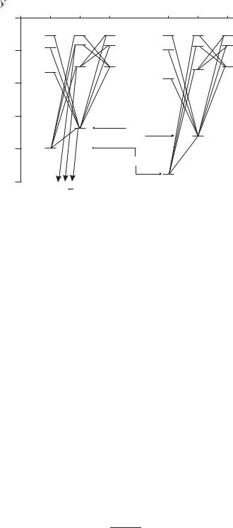
Fig. 3.4 The energy levels of the helium atom with those of hydrogen for comparison. The 1s2 ground configuration is tightly bound. For the excited configurations of helium the 1s-electron screens the outer electron from the nuclear charge so that the 1snl configurations in helium have similar energy to the shell with principal quantum number n in hydrogen. The hydrogenic levels are indicated on the right. The interval between the 1L and 3L terms (equal to twice the exchange integral) is clear for the 1s2s, 1s2p, 1s3s, 1s3p and 1s4s configurations but it is smaller for higher n and l.

to construct the symmetrised wavefunctions ψspaceA and ψspaceS .13 In this basis of eigenstates it is simple to calculate the e ect of the electrostatic

repulsion.

3.2.1Spin eigenstates

The electrostatic repulsion between the two electrons leads to the wave-

functions ψspaceS and ψspaceA in the excited states of the helium atom. The ground state is a special case where both electrons have the same spatial

wavefunction, so only a symmetric solution exists. We did not consider spin since electrostatic interactions depend on the charge of the particle, not their spin. Neither H0 nor H contains any reference to the spin of the electrons. Spin does, however, have a profound e ect on atomic wavefunctions. This arises from the deep connection between spin and the symmetry of the wavefunction of indistinguishable particles.14 Note that here we are considering the total wavefunction in the systems that includes both the spatial part (found in the previous section) and the spin. Fermions have wavefunctions that are antisymmetric with respect to particle-label interchange, and bosons have symmetric ones. As a consequence of this symmetry property, fermions and bosons fill up the levels of a system in di erent ways, i.e. they obey di erent quantum statistics.

Electrons are fermions so atoms have total wavefunctions that are antisymmetric with respect to permutation of the electron labels. This requires ψspaceS to associate with an antisymmetric spin function ψspinA , and the other way round:

3.2Excited states of helium 51

13For two electrons, swapping the

particle labels		twice	brings us		back
to where	we	started, so		ψ (1,	2) =
±ψ (2, 1).	Therefore		the two possible
			S	and −1 for
eigenvalues are 1 for ψspace

ψspaceA .

14Indistinguishable means that the particles are identical and have the freedom to exchange positions, e.g. atoms in a gas which obey Fermi–Dirac or Bose–Einstein statistics depending on their spin. In contrast, atoms in a solid can be treated as distinguishable, even if they are identical, because they have fixed positions—we could label the atoms 1, 2, etc. and still know which is which at some later time.

ψ = ψS	ψA	or	ψA	ψS .	(3.18)
space	spin		space	spin

These antisymmetrised wavefunctions that we have constructed fulfil the requirement of having particular symmetry with respect to the interchange of indistinguishable particles. Now we shall find the spin eigenfunctions explicitly. We use the shorthand notation where ↑ and ↓ represent ms = 1/2 and −1/2, respectively. Two electrons have four possible combinations: the three symmetric functions,

ψspinS = |↑↑
1			{ |↑↓ + |↓↑ }	(3.19)
= √
	2
= |↓↓ ,

	corresponding to S = 1 and MS = +1, 0, −1; and an antisymmetric
	function	1
	A
		= √2	{ |↑↓ − |↓↑ } ,	(3.20)
	ψspin

corresponding to S = 0 (with MS = 0).15 Spectroscopists label the eigenstates of the electrostatic interactions with the symbol 2S+1L, where S is the total spin and L is the total orbital angular momentum quantum number. The 1snl configurations in helium L = l, so the allowed terms

15These statements about the result of adding two s = 1/2 angular momenta can be proved by formal angular momentum theory. Simplified treatments describe S = 0 as having one electron with ‘spin-up’ and the other with ‘spin-down’; but both MS = 0 states are linear combinations of the states |ms1 = +1/2, ms2 = −1/2 and |ms1 = −1/2, ms2 = +1/2 .

52 Helium

16The letter ‘S’ appears over-used in this established notation but no ambiguity arises in practice. The symbol S for the total spin is italic because this is a variable, whereas the symbols S for L = 0 and s for l = 0 are not italic.

are 1L and 3L, e.g. the 1s2s configuration in helium gives rise to the terms 1S and 3S, where S represents L = 0.16

In summary, we have calculated the structure of helium in two distinct stages.

(1)Energies Degenerate perturbation theory gives the space wavefunctions ψspaceS and ψspaceA with energies split by twice the exchange integral. In helium the degeneracy arises because the two electrons are identical particles so there is exchange degeneracy, but the treatment is similar for systems where a degeneracy arises by accident.

(2)Spin We determined the spin associated with each energy level by constructing symmetrised wavefunctions. The product of the spatial functions and the spin eigenstates gives the total atomic wavefunction that must be antisymmetric with respect to particle-label interchange.

Exchange degeneracy, exchange integrals, degenerate perturbation theory and symmetrised wavefunctions all occur in helium and their interrelationship is not straightforward so that misconceptions abound. A common misinterpretation is to infer that because levels with di erent total spin, S = 0 and 1, have di erent energies then there is a spindependent interaction—this is not correct, but sometimes in condensed matter physics it is useful to pretend that it is! (See Blundell 2001.) The interactions that determine the gross structure of helium are entirely electrostatic and depend only on the charge and position of the particles. Also, degenerate perturbation theory is sometimes regarded as a mysterious quantum phenomenon. Appendix A gives further discussion and shows that symmetric and antisymmetric normal modes occur when two classical systems, with similar energy, interact, e.g. two coupled oscillators.

17This anticipates a more general discussion of this and other selection rules for the LS-coupling scheme in a later chapter.

3.2.2Transitions in helium

To determine which transitions are allowed between the energy levels of helium we need a selection rule for spin: the total spin quantum number does not change in electric dipole transitions. In the matrix element ψfinal|r|ψinitial the operator r does not act on spin; therefore, if the ψfinal and ψinitial do not have the same value of S, then their spin functions are orthogonal and the matrix element equals zero.17 This selection rule gives the transitions shown in Fig. 3.5.

3.3 Evaluation of the integrals in helium 53

	−
	−
		Fig. 3.5 The allowed transitions be-
	−	tween the terms of helium are governed
		by the selection rule ∆S = 0 in addi-
		tion to the rule ∆l = ±1 found pre-
		viously. Since there are no transitions
	−	between singlets and triplets it is con-
		venient to draw them as two separate
		systems. Notice that in the radiative
		decay of helium atoms excited to high-
	−	lying levels there are bottlenecks in the
		metastable 1s2s 1S and 1s2s 3S terms.

3.3Evaluation of the integrals in helium

In this section we shall calculate the direct and exchange integrals to make quantitative predictions for some of the energy levels in the helium atom, based on the theory described in the previous sections. This provides an example of the use of atomic wavefunctions to carry out a calculation where there are no corresponding classical orbits and gives an indication of the complexities that arise in systems with more than one electron. The evaluation of the integrals requires care and some further details are given in Appendix B. The important point to be learnt from this section, however, is not the mathematical techniques but rather to see that the integrals arise from the Coulomb interaction between electrons treated by straightforward quantum mechanics.

3.3.1Ground state

To calculate the energy of the 1s2 configuration we need to find the expectation value of e2/4π 0r12 in eqn 3.1—this calculation is the same as the evaluation of the mutual repulsion between two charge distributions in classical electrostatics, as in eqn 3.15 with ρ1s(r1) and ρnl(r2) = ρ1s(r2). The integral can be considered in di erent ways. We could calculate the energy of the charge distribution of electron 1 in the potential created by electron 2, or the other way around. This section does neither; it uses a method that treats each electron symmetrically (as in Appendix B), but of course each approach gives the same numerical result. Electron 1 produces an electrostatic potential at radial distance r2 given by

r2	1
V12 (r2) = 0 4π 0r12		ρ(r1) d3r1 .	(3.21)

54 Helium

18Here Q (∞) = −e.

19As is usual in calculations of the interaction between electric charge distributions, one must be careful to avoid double counting. This method of calculation avoids this pitfall, as shown by the general argument in Appendix B. An alternative method is used in Woodgate (1980), Problem 5.5.

The spherical symmetry of s-electrons means that the charge in the region r1 < r2 acts like a point charge at the origin, so that

V12 (r2) = Q (r2) ,

4π 0r2

where Q (r2) is the charge within a radius of r2 from the origin, which is given by18

Q (r2) = 0		r2
		ρ (r1) 4πr12 dr1 .	(3.22)
The electrostatic energy that arises from the repulsion equals
E12 = 0	∞
	V12 (r2) ρ (r2) 4πr22 dr2 .		(3.23)

For the 1s2 configuration there is an exactly equal contribution to the energy from V21 (r1), the (partial) potential at r1 produced by electron 2. Thus the total energy of the repulsion between the electrons is twice that in eqn 3.23.19 Using the radial wavefunction for a 1s-electron, we find

J1s2 =

2× 4π 0

0

∞

0

r1

4Z3e−(Z/a0 )2r1 r12 dr1

4Z3e−(Z/a0 )2r2 r22 dr2

e2

r2

1

e2/4π 0 5

5

=

Z = (13.6 eV) ×

Z .

(3.24)

2a0

4

4

For helium this gives J1sZ=22 = 34 eV.

20The e ect of the repulsion proportional to 1/r12 can be considered in terms of potentials like that in eqn 3.21 (and Appendix B). The potential at the position of the outer electron r2 arising from the charge distribution of electron 1 accounts for a large portion of the total repulsion: V12(r2)

e2/4π 0r2 in the region where ρnl (r2) has an appreciable value. Hence it

makes sense to include e2/4π 0r2 in the zeroth-order Hamiltonian H0a and treat the (small) part left over as a perturbation Ha.

3.3.2Excited states: the direct integral

A 1snl configuration of helium has an energy close to that of an nl- electron in hydrogen, e.g. in the 1s2p configuration the 2p-electron has a similar binding energy to the n = 2 shell of hydrogen. The obvious explanation, in Bohr’s model, is that the 2p-electron lies outside the 1sorbit so that the inner electron screens the outer one from the full nuclear charge. Applying an analogous argument to the quantum treatment of helium leads to the Hamiltonian H = H0a + Ha, where20

2

e2

2

1

H0a = −

12 + 22 −

+

(3.25)

2m

4π 0

r1

r2

and

e2

1

1

Ha

=

−

.

(3.26)

4π 0

r12

r2

In the expression for H0a, electron 2 experiences the Coulomb attraction of a charge +1e. In Ha the subtraction of e2/4π 0r2 from the mutual repulsion means that the perturbation tends to zero at a large distance from the nucleus (which is intuitively reasonable). This decomposition di ers from that in Section 3.1. The di erent treatment of the two electrons makes the perturbation theory a little tricky, but Heisenberg

3.3 Evaluation of the integrals in helium 55

did the calculation as described in Bethe and Salpeter (1957) or Bethe

and Salpeter (1977); he found the direct integral

J1snl

= 4π 0

r12 − r2

|u1s(1)|2 |unlm(2)|2 d3r1 d3r2 .

(3.27)

e2

1

1

This must be evaluated with the appropriate wavefunctions, i.e. uZ=1

nlm

rather than unlmZ=2, and u1sZ=2 as before.21 For the excited electron unlm =

21We have not derived this integral rig-

Rnl(r)Ylm (θ, φ), where Rnl(r) is the radial function for Z = 1. We write

orously but it has an intuitively reason-

the direct integral as

able form.

e2

∞

∞

J1snl =

0

0

J(r1, r2) R102 (r1)Rnl2 (r2)r12 dr1 r22 dr2 ,

(3.28)

4π 0

22

22

√

Y00

4π.

where the angular parts are contained in the function

(θ1, φ1) = 1/

2π

π

2π

π

1

1

1

J(r1, r2) = 0

0

0

0

−

|Ylm(θ2, φ2)|2

(3.29)

r12

r2

4π

× sin θ1 dθ1 dφ1 sin θ2 dθ2 dφ2 .

The calculation of this integral requires the expansion of 1/r12 in terms

of spherical harmonics:23

23Y

(θ1, φ1) = (

−

1)q Yk,

−

q (θ1, φ1).

1

1

∞

r1

4π

k,q

k

k

r12

=

r2

k=0

r2

2k + 1

q=

−

k Yk,q (θ1, φ1) Yk,q (θ2, φ2)

(3.30)

for r2

> r

r

1 ↔

r

when r1

> r2). Only the

term for k = 0

1 (and

2

24

24

When k

= 0 the integral of the func-

survives in the integration over angles in eqn 3.29 to give

0

for r1 < r2 ,

tion Yk,q (θ1, φ1) over θ1 and φ1 equals

1/r2

zero.

J(r1, r2) = 1/r1

−

for r1 > r2 .

When r1 < r2 the original screening argument applies and eqn 3.25 gives a good description. When r1 > r2 the appropriate potential is proportional to −2/r2 − 1/r1 and J(r1, r2) accounts for the di erence between this and −2/r1 − 1/r2 used in H0a. Thus we find

J1snl = 4π 0 0		r2	r1	− r2		R102 (r1)r12 dr1 Rnl2 (r2)r22 dr2 .
	e2	∞ ∞	1	1

(3.31) Evaluation of this integral for the 1s2p configuration (in Exercise 3.6) gives J1s2p = −2.8 × 10−2 eV—three orders of magnitude smaller than J1sZ=22 in eqn 3.7 (evaluated from eqn 3.24). The unperturbed wavefunction for Z = 1 has energy equal to that of the corresponding level in hydrogen and the small negative direct integral accounts for the incompleteness of the screening of the nl-electron by the inner electron.

3.3.3Excited states: the exchange integral

The exchange integral has the same form as eqn 3.16 but with uZnlm=1 rather than uZnlm=2 (and uZ1s=2 as before). Within the spatial wavefunction