Atomic physics (2005)

36 The hydrogen atom

(a)

(b)

Fig. 2.3 The representation of (a) spinup and (b) spin-down states as vectors precessing around the z-axis.

45The Biot–Savart law for the magnetic field from a current flowing along a straight wire can be recovered from the Lorentz transformation and Coulomb’s law (Gri ths 1999). However, this link can only be made in this direction for simple cases and generally the phenomenon of magnetism cannot be ‘derived’ in this way.

a structureless elementary particle with no measurable size. So we are left with the experimental fact that the electron has an intrinsic spin angular momentum of /2 and these half-integer values are perfectly acceptable within the general theory of angular momentum in quantum mechanics.

2.3.2The spin–orbit interaction

The Schr¨odinger equation is non-relativistic, as can readily be seen by looking at the kinetic-energy operator that is equivalent to the nonrelativistic expression p2/2me. Some of the relativistic e ects can be taken into account as follows. An electron moving through an electric field E experiences an e ective magnetic field B given by

1	(2.45)
B = −c2 v × E .

This is a consequence of the way an electric field behaves under a Lorentz transformation from a stationary to a moving frame in special relativity. Although a derivation of this equation is not given here, it is certainly plausible since special relativity and electromagnetism are intimately linked through the speed of light c = 1/√ 0µ0. This equation for the speed of electromagnetic waves in a vacuum comes from Maxwell’s equations; 0 being associated with the electric field and µ0 with the magnetic field. Rearrangement to give µ0 = 1/ 0c2 suggests that magnetic fields arise from electrodynamics and relativity.45

We now manipulate eqn 2.45 into a convenient form, by substituting for the electric field in terms of the gradient of the potential energy V and unit vector in the radial direction:

E =	1		∂V		r	.	(2.46)
	e
			∂r r

The factor of e comes in because the electron’s potential energy V equals its charge −e times the electrostatic potential. From eqn 2.45 we have

B =

1

1 ∂V

r × mev =

1 ∂V

l ,

(2.47)

mec2

er

∂r

mec2

er

∂r

where the orbital angular momentum is l = r × mev. The electron has an intrinsic magnetic moment µ = −gsµBs, where the spin has a magnitude of |s| = s = 1/2 (in units of ) and gs 2, so the moment

2.3 Fine structure 37

has a magnitude close to one Bohr magneton (µB = e /2me). The interaction of the electron’s magnetic moment with the orbital field gives the Hamiltonian

	H = −µ · B			1 ∂V			l .
	= gsµBs ·							(2.48)
		mec2		er		∂r

However, this expression gives energy splittings about twice as large as observed. The discrepancy comes from the Thomas precession—a relativistic e ect that arises because we are calculating the magnetic field in a frame of reference that is not stationary but rotates as the electron moves about the nucleus. The e ect is taken into account by

46

find the spin–orbit interaction,

replacing gs with gs −1 1. Finally, we

47

including the Thomas precession factor, is

2

1 ∂V

Hs−o = (gs − 1)

s · l .

(2.49)

2me2c2

r

∂r

For the Coulomb potential in hydrogen we have

1 ∂V

=

e2/4π 0

.

(2.50)

r ∂r

r3

The expectation value of this Hamiltonian gives an energy change of48

	2		e2	1
Es−o =						s · l .	(2.51)
	2me2c2		4π 0		r3

The separation into a product of radial and angular expectation values

followsfrom the separability of the wavefunction. The integral 1/r3 is

given in eqn 2.23. However, we have not yet discussed how to deal with interactions that have the form of dot products of two angular momenta; let us start by defining the total angular momentum of the atom as the sum of its orbital and spin angular momenta,

j = l + s .

(2.52)

This is a conserved quantity for a system without any external torque acting on it, e.g. an atom in a field-free region of space. This is true both in classical and quantum mechanics, but we concentrate on the classical explanation in this section. The spin–orbit interaction between l and s causes these vectors to change direction, and because their sum is constrained to be equal to j they move around as shown in Fig. 2.4.49 Squaring and rearranging eqn 2.52, we find that 2 s · l = j2 − l2 − s2.

Hence we can find the expectation value in terms of the known values
for j2 ,	l2	and s2 1as
		s · l =				{j (j + 1)	− l (l + 1) − s (s + 1)} .	(2.53)
				2
Thus the spin–orbit interaction produces a shift in energy of
			β
		Es−o =			{j (j + 1)		− l (l + 1) − s (s + 1)} ,	(2.54)
			2

46This is almost equivalent to using gs/2 1, but gs − 1 is more accurate at the level of precision where the small deviation of gs from 2 is important (Haar and Curtis 1987). For further discussion of Thomas precession see Cowan (1981), Eisberg and Resnick (1985) and Munoz (2001).

47We have derived this classically, e.g. by using l = r × mev. However, the same expression can be obtained from the fully relativistic Dirac equation for an electron in a Coulomb potential by making a low-velocity approximation, see Sakurai (1967). That quantum mechanical approach justifies treating l and s as operators.

48Using the approximation gs − 1 1.

s

l

j

Fig. 2.4 The orbital and spin angular momenta add to give a total atomic angular momentum of j.

49In this precession about j the magnitudes of l and s remain constant. The magnetic moment (proportional to s) is not altered in an interaction with a magnetic field, and because of the symmetrical form of the interaction in eqn 2.49, we do not expect l to behave any di erently. See also Blundell (2001) and Section 5.1.

38 The hydrogen atom

where the spin–orbit constant β is (from eqns 2.51 and 2.23)

β =	2		e2	1			.	(2.55)
	2me2c2		4π 0		(na0)3 l l + 21	(l + 1)

A single electron has s = 12 so, for each l, its total angular momentum quantum number j has two possible values:

j = l +	1	or l −	1	.
	2		2

From eqn 2.54 we find that the energy interval between these levels, ∆Es−o = Ej=l+ 12 − Ej=l− 12 , is

∆Es−o = β l +	1		=	α2hcR∞
	2			n3l (l + 1)	.

50As shown in Section 1.9, meαca0 = Or, expressed in terms of the gross energy E(n) in eqn 1.10,50

and hcR∞ = (e2/4π 0)/(2a0 ).		α2
	∆Es−o =		E (n) .
		n l (l + 1)

(2.56)

(2.57)

This agrees with the qualitative discussion in Section 1.4, where we showed that relativistic e ects cause energy changes of order α2 times the gross structure. The more complete expression above shows that the energy intervals between levels decrease as n and l increase. The largest interval in hydrogen occurs for n = 2 and l = 1; for this configuration the spin–orbit interaction leads to levels with j = 1/2 and j = 3/2. The full designation of these levels is 2p 2P1/2 and 2p 2P3/2, in the notation that will be introduced for the LS-coupling scheme. But some of the quantum numbers (defined in Chapter 5) are superfluous for atoms with a single valence electron and a convenient short form is to denote these two levels by 2 P1/2 and 2 P3/2; these correspond to n Pj , where P represents the (total) orbital angular momentum for this case. (The capital letters are consistent with later usage.) Similarly, we may write

2 S1/2 for the 2s 2S1/2 level; 3 D3/2 and 3 D5/2 for the j = 3/2 and 5/2 51Another short form found in the lit- levels, respectively, that arise from the 3d configuration.51 But the full erature is 2 2P1/2 and 2 2P3/2. notation must be used whenever ambiguity might arise.

2.3.3The fine structure of hydrogen

As an example of fine structure, we look in detail at the levels that arise from the n = 2 and n = 3 shells of hydrogen. Equation 2.54 predicts that, for the 2p configuration, the fine-structure levels have energies of

Es−o		2 P1/2			= −β2p ,
E		2 P	3/2		= 1		β		2p	,
s−o					2
as shown in Fig. 2.5(a). For the 3d configuration
Es−o	3 D3/2				= −		3	β3d			,
							2
E	3 D				= β	3d			,
s−o		5/2

2.3 Fine structure 39

as shown in Fig. 2.5(b). For both configurations, it is easy to see that	(a)
the spin–orbit interaction does not shift the mean energy

	= (2j + 1) Ej (n, l) + (2j + 1) Ej (n, l) ,	(2.58)
E

where j = l − 1/2 and j = l + 1/2 for the two levels. This calculation of the ‘centre of gravity’ for all the states takes into account the degeneracy of each level.

The spin–orbit interaction does not a ect the 2 S1/2 or 3 S1/2 so we might expect these levels to lie close to the centre of gravity of the configurations with l > 0. This is not the case. Fig. 2.6 shows the energies of the levels for the n = 3 shell given by a fully relativistic calculation. We can see that there are other e ects of similar magnitude to the spin–orbit interaction that a ect these levels in hydrogen. Quite remarkably, these additional relativistic e ects shift the levels by just the right amount to make n P1/2 levels degenerate with the n S1/2 levels, and n P3/2 degenerate with n D3/2. This structure does not occur by chance, but points to a deeper underlying cause. The full explanation of these observations requires relativistic quantum mechanics and the technical details of such calculations lie beyond the scope of this book.52 We shall simply quote the solution of the Dirac equation for an electron in a Coulomb potential; this gives a formula for the energy EDirac (n, j) that depends only on n and j, i.e. it gives the same energy for levels of the same n and j but di erent l, as in the cases above. In a comparison of the

No spin−orbit interaction

(b)

No spin−orbit interaction

Fig. 2.5 The fine structure of hydrogen. The fine structure of (a) the 2p and (b) the 3d configurations are drawn on di erent scales: β2p is considerably greater than β3d. All p- and d- configurations look similar apart from an overall scaling factor.

52See graduate-level quantum mechanics texts, e.g. Sakurai (1967) and Series (1988).

S			P					D
			Non-relativistic limit
								Relativistic
			Relativistic					mass
Relativistic			mass						Spin−orbit
mass
				Spin−orbit

Darwin term for s-electrons

Fig. 2.6 The theoretical positions of the energy levels of hydrogen calculated by the fully relativistic theory of Dirac depend on n and j only (not l), as shown in this figure for the n = 3 shell. In addition to the spin–orbit interaction, the e ects that determine the energies of these levels are: the relativistic mass correction and, for s-electrons only, the Darwin term (that accounts for relativistic e ects that occur at small r, where the electron’s momentum becomes comparable to mec).

40 The hydrogen atom

53The Dirac equation predicts that the electron has gs = 2 exactly.

exact relativistic solution of the Dirac equation and the non-relativistic energy levels, three relativistic e ects can be distinguished.

(a)There is a straightforward relativistic shift of the energy (or equivalently mass), related to the binomial expansion of γ = (1−v2/c2)−1/2, in eqn 1.16. The term of order v2/c2 gives the non-relativistic ki-

netic energy p2/2me. The next term in the expansion is proportional to v4/c4 and gives an energy shift of order v2/c2 times the gross structure—this is the e ect that we estimated in Section 1.4.

(b)For electrons with l = 0, the comparison of the Dirac and Schr¨odinger equations shows that there is a spin–orbit interaction of the form given above, with the Thomas precession factor naturally included.53

(c)For electrons with l = 0 there is a Darwin term proportional to |ψ (r = 0)|2 that has no classical analogue (see Woodgate (1980) for further details).

That these di erent contributions conspire together to perturb the wavefunctions such that levels of the same n and j are degenerate seems improbable from a non-relativistic point of view. It is worth reiterating the statement above that this structure arises from the relativistic Dirac equation; making an approximation for small v2/c2 shows that these three corrections, and no others, need to be applied to the (nonrelativistic) energies found from the Schr¨odinger equation.

54Lamb and Retherford used a radiofrequency to drive the 2 S1/2–2 P1/2 transition directly. This small energy interval, now know as the Lamb shift, cannot be resolved in conventional spectroscopy because of Doppler broadening, but it can be seen using Doppler-free methods as shown in Fig. 8.7.

55The QED calculation of the Lamb shift is described in Sakurai (1967).

56Broadly speaking, in a mathematical treatment these vacuum fluctuations correspond to the zero-point energy of quantum harmonic oscillators, i.e. the lowest energy of the modes of the system is not zero but ω/2.

57QED also explains why the g-factor of the electron is not exactly 2. Precise measurements show that gs = 2.002 319 304 371 8 (current values for the fundamental constants can be found on the NIST web site, and those of other national standards laboratories). See also Chapter 12.

2.3.4The Lamb shift

Figure 2.7 shows the actual energy levels of the n = 2 and n = 3 shells. According to relativistic quantum theory the 2 S1/2 level should be exactly degenerate with 2 P1/2 because they both have n = 2 and j = 1/2, but in reality there is an energy interval between them, E 2 S1/2 −

E 2 P1/2	1 GHz. The shift of the 2 S1/2 level to a			higher energy
(lower binding energy) than the E		Dirac	(n = 2, j = 1/2) is about one-

tenth of the interval between the two fine-structure levels, E 2 P3/2 −

E 2 P			11 GHz. Although small, this discrepancy in	hydrogen was
	1/2
of great		historical importance in physics. For this simple one-electron

atom the predictions of the Dirac equation are very precise and that theory cannot account for Lamb and Retherford’s experimental measurement that the 2 S1/2 level is indeed higher than the 2 P1/2 level.54 The explanation of this Lamb shift goes beyond relativistic quantum mechanics and requires quantum electrodynamics (QED)—the quantum field theory that describes electromagnetic interactions. Indeed, the observation of the Lamb shift experiment was a stimulus for the development of this theory.55 An intriguing feature of QED is so-called vacuum fluctuations—regions of free space are not regarded as being completely empty but are permeated by fluctuating electromagnetic fields.56 The QED e ects lead to a significant energy shift for electrons with l = 0 and hence break the degeneracy of 2 S1/2 and 2 P1/2.57 The largest QED shift occurs for the 1 S1/2 ground level of hydrogen but there is no other level nearby and so a determination of its energy requires a precise mea-

2.3 Fine structure 41

Spin−orbit

Lamb shift

(a)

(b)

(c)

Fig. 2.7 The fine structure of the n = 2 and n = 3 shells of hydrogen and the allowed transitions between the levels. According to the Dirac equation, the 2 S1/2 and 2 P1/2 levels should be degenerate, but they are not. The measured positions show that the 2s 2S1/2 level is shifted upwards relative

to the position EDirac (n = 2, j = 1/2) and is therefore not degenerate with

the 2p 2P1/2 level. Such a shift occurs for all the s-electrons (but the size of the energy shift decreases with increasing n). The explanation of this shift takes us beyond relativistic quantum mechanics into the realm of quantum electrodynamics (QED)—the quantum field theory that describes electromagnetic interactions.

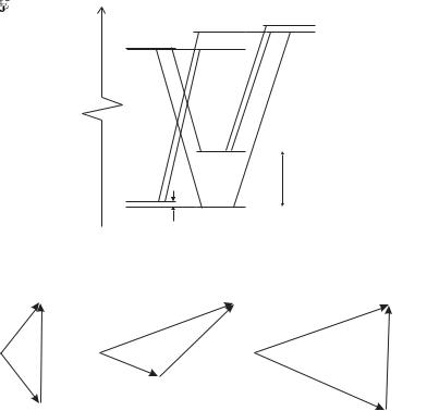
Fig. 2.8 The conservation of total angular momentum in electric dipole transitions that gives the selection rule in eqn 2.59 can be represented as vector addition. The photon has one unit of angular momentum, and so to go from level j1 to j2 the vectors must form a triangle, as shown for the case of (a) j1 = 1/2 to j2 = 1/2, (b) j1 = 1/2 to j2 = 3/2 and (c) j1 = 3/2 to j2 = 3/2.

surement of a large frequency. Nowadays this can be achieved by laser spectroscopy (Chapter 8) but the near degeneracy of the two j = 1/2 levels with n = 2 was crucial in Lamb’s experiment.58 Another important feature in that experiment was the metastability of the 2 S1/2 level, whose lifetime was given in Section 2.2.3. That level decays 108 times more slowly than that of 2 P1/2. In an atomic beam of hydrogen (at room temperature) the atoms have typical velocities of about 3000 m s−1 and atoms excited into the 2p configuration travel an average distance of only 5 × 10−6 m before decaying with the emission of Lyman-α radiation. In contrast, metastable atoms travel the full length of the apparatus ( 1 m) and are de-excited when they collide with a detector (or the wall of the vacuum chamber). Hydrogen, and hydrogenic systems, are still used for experimental tests of fundamental theory because their simplicity allows very precise predictions.

58Higher shells have smaller shifts between the j = 1/2 levels.

2.3.5Transitions between fine-structure levels

Transitions in hydrogen between the fine-structure levels with principal quantum numbers n = 2 and 3 give the components of the Balmer-α line shown in Fig. 2.7; in order of increasing energy, the seven allowed

42 The hydrogen atom

transitions between the levels with di erent j are as follows:

2 P3/2 − 3 S1/2 , 2 P3/2 − 3 D3/2 , 2 P3/2 − 3 D5/2 , 2 S1/2 − 3 P1/2 , 2 P1/2 − 3 S1/2 , 2 S1/2 − 3 P3/2 , 2 P1/2 − 3 D3/2 .

These obey the selection rule ∆l = ±1 but an additional rule prevents a transition between 2 P1/2 and 3 D5/2, namely that the change of the total angular momentum quantum number in an electric dipole transition obeys

∆j = 0, ±1.

(2.59)

This selection rule may be explained by angular momentum conservation (as mentioned in Section 2.2.2). This rule can be expressed in terms of vector addition, as shown in Fig. 2.8; the conservation condition is equivalent to being able to form a triangle from the three vectors representing j of the initial state, the final state, and a unit vector for the (one unit of) angular momentum carried by the photon. Hence, this selection rule is sometimes referred to as the triangle rule. The projection of j along the z-axis can change by ∆mj = 0, ±1. (Appendix C gives a summary of all selection rules.)

Further reading

Much of the material covered in this chapter can be found in the introductory quantum mechanics and atomic physics texts listed in the References. For particular topics the following are useful: Segr` (1980) gives an overview of the historical development, and Series (1988) reviews the work on hydrogen, including the important Lamb shift experiment.

Exercises

(2.1) Angular-momentum eigenfunctions		(2.2) Angular-momentum eigenfunctions
(a)	Verify that all the eigenfunctions with l = 1	(a)	Find the eigenfunction with orbital angular
	are orthogonal to Y0,0.		momentum quantum number l and magnetic
(b)	Verify that all the eigenfunctions with l = 1		quantum number m = l − 1.
	are orthogonal to those with l = 2.	(b)	Verify that Yl,l−1 is orthogonal to Yl−1,l−1.

Exercises for Chapter 2

43

(2.3)

Radial wavefunctions

wavefunction

Verify eqn 2.23 for n = 2, l = 1 by calculating the

−iE1t/

−iE2t/

.

radial integral (for Z = 1).

Ψ (t) = Aψ1 (r) e

+ Bψ2 (r) e

(2.4)

Hydrogen

The distribution of electronic charge is given by

For a hydrogen atom the normalised wavefunction

e Ψ (t) 2

=

e

Aψ1

2 + Bψ2

2

of an electron in the 1s state, assuming a point

−

|

|

−

+|

|

2A| Bψ|1 ψ2

|cos (ω12t

−

φ) .

nucleus, is

|

Part of this oscillates at the (angular) frequency

1

1/2

of the transition ω12 = ω2 − ω1 = (E2 − E1) / .

e−r/a0 ,

ψ(r) =

3

πa0

(a)

A hydrogen atom is in a superposition of the

where a0 is the Bohr radius. Find an approximate

1s ground state, ψ1 = R1,0 (r) Y0,0 (θ, φ), and

the ml

= 0 state of the 2p configuration, ψ2 =

expression for the probability of finding the elec-

R2,1 (r) Y1,0 (θ, φ);

A 0.995

and B

=

0.1

tron in a small sphere of radius rb

a0 centred on

(so the term containing B2

can be ignored).

the proton. What is the electronic charge density

Sketch the form of the charge distribution for

in this region?

one cycle of oscillation.

(2.5)

Hydrogen

(b)

The atom in a superposition state may have

The Balmer-α spectral

line

is observed from a

an oscillating electric dipole moment

(weak) discharge in a lamp that contains a mixture

of hydrogen and deuterium at room temperature.

−eD (t) = −e Ψ

(t) rΨ (t) .

Comment on the feasibility of carrying out an ex-

periment using a Fabry–Perot ´etalon to resolve (a)

What are

the conditions on ψ1 and ψ2

for

which D (t) = 0.

the isotope shift, (b) the fine structure and (c) the

Lamb shift.

(c)

Show that an atom in a superposition of the

(2.6)

Transitions

same states as in part (a) has a dipole moment

of

Estimate the lifetime of the excited state in a two-

level atom when the transition wavelength is (a)

−eD (t) = −e |2A

B| Iang

100 nm and (b) 1000 nm. In what spectral regions

do these wavelengths lie?

× rR2,1(r)R1,0(r)r2 dr cos(ω12t)ez ,

(2.7)

Selection rules

where

is an integral with respect to θ and

ang

By explicit calculation of integrals over θ, for the

I

case of π-polarization only, verify that p to d tran-

φ. Calculate the amplitude of this dipole, in

units of ea0, for A = B = 1/√2.

sitions are allowed, but not s to d.

(2.8)

Spin–orbit interaction

(d)

A hydrogen atom is in a superposition of the

1s ground state and the ml

= 1 state of the 2p

The spin–orbit interaction splits a single-electron

configuration, ψ2 = R2,1 (r) Y1,1 (θ, φ). Sketch

configuration into two

levels

with total angular

the form of the charge distribution at various

momentum quantum numbers j

= l + 1/2 and

points in its cycle of oscillation.

j = l − 1/2. Show that this interaction does not

shift the mean energy (centre of gravity) of all the

(e)

Comment on the relationship between the

states given by (2j + 1) Ej + (2j + 1) Ej .

time dependence of the charge distributions

(2.9)

Selection rule for the magnetic quantum number

sketched in this exercise and the motion of the

electron in the classical model of the Zeeman

Show that the angular integrals for σ-transitions

e ect (Section 1.8).

contain the factor

2π

(2.11)

Angular eigenfunctions

0

i(ml1

−

ml2

±

1)φ

We shall find the angular momentum eigenfunc-

e

dφ .

tions using ladder operators, by assuming that for

Hence derive the selection rule ∆ml = ±1 for this

some value of l there is a maximum value of the

magnetic quantum number mmax.

For this case

polarization. Similarly, derive the selection rule

Yl,mmax Θ(θ)eimmaxφ and the function Θ(θ) can

for the π-transitions.

(2.10)

Transitions

be found from

An atom in a superposition of two states has the

l+Θ(θ) exp (immaxφ) = 0 .

44 The hydrogen atom

(a) Show that Θ(θ) satisfies the equation

Hence, or otherwise, prove that Iang is zero unless

1

∂Θ(θ)

cos θ

the initial and final states have opposite parity.

= mmax

.

Θ(θ)

∂θ

sin θ

(2.13)

Selection rules in hydrogen

(b) Find the solution

of

the equation for

Θ(θ).

Hydrogen atoms are excited (by a pulse of laser

light that drives a multi-photon process) to a spe-

(Both sides have the form f (θ)/f (θ) whose

cific configuration and the subsequent spontaneous

integral is ln{f (θ)}.)

By

substituting

emission is resolved using a spectrograph. Infra-

this solution

into

eqn

2.5 to

show

that

red and visible spectral lines are detected only at

b = mmax(mmax + 1),

or otherwise,

obtain

the wavelengths 4.05 µm, 1.87 µm and 0.656 µm.

eqn 2.10.

Explain these observations and give the values of

(2.12) Parity and selection rules

that l2 − l1

n and l for the configurations involved in these

Show that eqn 2.42 implies

is odd.

transitions.

Web site:

http://www.physics.ox.ac.uk/users/foot

This site has answers to some of the exercises, corrections and other supplementary information.

Helium	3

Helium has only two electrons but this simplicity is deceptive. To treat systems with two particles requires new concepts that also apply to multi-particle systems in many branches of physics, and it is very worthwhile to study them carefully using the example of helium. There is truth in the saying that atomic physicists count ‘one, two, many’ and a detailed understanding of the two-electron system is su cient for much of the atomic structure in this book.1

3.1The ground state of helium

Two electrons in the Coulomb potential of a charge Ze, e.g. the nucleus of an atom, obey a Schr¨odinger equation of the form

− 2

2

+

− 2

2

+

e2

Z

Z

+

1

ψ = Eψ . (3.1)

4π 0

−r1

r12

2m 1

2m 2

− r2

Here r12 = |r1 − r2| is the distance between electron 1 and electron 2 and the electrostatic repulsion of electrons is proportional to 1/r12. Neglecting this mutual repulsion for the time being, we can write the equation as

(H1 + H2) ψ = E(0)ψ ,							(3.2)
where			− 2			Z e2
H		≡		2	−		(3.3)
						4π 0r1
	1		2m 1

and H2 is a similar expression for electron 2. Writing the atomic wavefunction as a product of the wavefunctions for each electron, ψ = ψ (1) ψ (2), allows us to separate eqn 3.2 into two single-electron Schr¨odinger equations:

H1ψ (1) = E1ψ (1)

(3.4)

and a similar equation for ψ (2) with energy E2. The solutions of these one-electron equations are hydrogenic wavefunctions with energies given by the Rydberg formula. Helium has Z = 2 and in its ground state both electrons have energy E1 = E2 = −4hcR∞ = −54.4 eV. Thus the total energy of the atom (neglecting repulsion) is

E(0) = E1 + E2 = −109 eV .

(3.5)

3.1	The ground state of helium 45
3.2	Excited states of helium	46
3.3	Evaluation of the integrals
	in helium	53
Further reading		56
Exercises		58

1This book considers only those multielectron systems with one, or two, valence electrons ‘outside’ a sphericallysymmetric core of charge.