Laboratory work 4 Systematic convolutional codes correcting capability research

Objective: To determinate the quality parameters of the system with the error-correction coding by convolutional code (14, 7) with a threshold algorithm decoding in a channel with additive white Gaussian noise (AWGN).

Laboratory emulator:

After opening the file “Project1.exe” you can see interface like fig. 3.6.

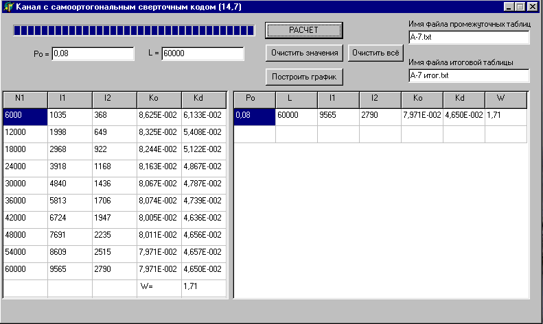
Figure 3.6 – The interface of laboratory work

You need enter the data from table 3.6, where p₀ – error probability, L – amount of codewords.

Table 3.6 – Results of coding gain by error probability in the DSC

p0	0,07	0,05	0,03	0,01	0,005	0,003
L	25·10^4	5·10^5	75·10^4	10^6	4·10^6	5·10^6
Wep

In the result of the experiment, you get next parameters:

• i1 – amount of errors in the discrete symmetric channel (DSC);

• i2 – amount of uncorrected errors by the decoder;

• k₀ – errors coefficient in the DSC, k₀ nearly equal p₀;

• k_d – errors coefficient in the output of the decoder;

• W – coding gain.

These parameters are calculated by formulas:

k₀ =i1/2L, k_d =i2/L, W= k₀/k_d.

Then you can get the diagram k_d1 = f₀(p₀) after putting the button “Построить график”, as shown in fig. 3.7a.

For building of the diagram for determination of coding gain W in the channel with AWGN it is need to use two subsidiary diagrams in the fig 3.7b. The first diagram is the characteristic of the channel with PM-2 without coding . The second diagram with the double energy of the bit (as the relative information transfer rate R = ½).

p₀ 10^–3 10^–2 Р₀₁ 10^-1 10⁰ 0 1 2 h₁ 3 h

p₀ = f₂( h)

k_d =p₀

k_d2= f₃ ( h) p₀ =f₁( h)

k_d k_d, p₀

а) b)

Figure 3.7 – The characteristic of the DSC and the channel with AWGN

For example, for given value p₀₁ we can determinate the signal/noise ratio h₁ using the path 1→2→3→4. The value h₁ corresponds to error probability p₀₁ in the output of the PM-2 demodulator. Take to account that there is convolutional decoder (14, 7) before PM-2 demodulator, which decreases error probability p₀ in W times. That’s why the place of the point A on the diagram k_d2 = f₃( h) is determined using the paths 1→5→6→7 and 4→8. For getting the characteristic k_d2 it is need to use some values of p₀.

Laboratory task:

1. To open the file “Project1.exe”.

2. To enter initial data from the table 3.6 and fill it.

3. To draw the characteristic k_d1 = f₀ (p₀).

4. To build the graph k_d2 = f₃( h) using the values p₀ from the table 3.6.

5. To determine the value h_lim when the convolutional code (14, 7) is reasonable.

Home task:

1. To learn items 1.3.1 – 1.3.2 of this teaching manual.

2. To write down the answers to the general questions.

3. To prepare the table 3.6 in the protocol.

4. To prepare blank using Application B.

General questions:

1. What does the characteristic k_d1 = f₀ (p₀) describe?

2. What does the characteristic k_d2 = f₃( h) describe?

3. Determinate the coding gain by error probability W_ep = p₃/p₄, where p₃ – error probability in the channel without coding, p₄ – with coding, if h = 2,1 and 2,3 using the diagram 3.7b.

Protocol content:

1. Subject and objective.

2. Executed home task.

3. Graph and table according to laboratory task.

4. Conclusion. Compare two characteristics of k_d1 = f₀(p₀) and k_d = f(p₀) from the laboratory work 2.