SPE-118703-MS

SPE 118703	11

Laboratory Procedures

Vertical core samples were obtained from whole core samples, faced to a right cylinder, and tested at the “as received” saturation. Each sample was inserted into a rubber jacket and a radial Linear Variable Displacement Transducer (LVDT) was placed around the lateral surface of the sample. The sample was mounted between pistons with ports on the contacting surfaces for controlling pore pressure, and acoustic crystals for acquiring the sonic travel time. All samples reported here were tested at 0 psi imposed pore pressure and room temperature. The entire assembly was mounted in a pressure vessel that allows application of confining pressure and axial stress. The top piston extends through the top of the pressure vessel enabling the application of axial load. The pressure vessel was then loaded into a computer-controlled load frame where another LVDT was attached for axial strain measurements. The net reservoir stress was calculated for each sample using the initial reservoir pressure, overburden stress, and the estimated mechanical properties. The confining and axial pressures were increased at the same rate to the computed net confining pressure. The low axial stress sonic measurement was obtained at that point. Data logging was begun and the axial and radial strain were measured as the axial load was increased while holding the confining pressure constant. At near maximum axial stress, the high axial stress sonic velocity was again determined.

Static and Dynamic Poisson’s Ratio

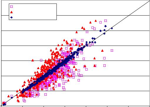
Figure 8 shows the variation in Poisson’s Ratio derived using the high axial stress acoustic measurements compared to those derived at low stress. The dashed line shows the 1:1 relationship. The data show that there is no first order correction for stress state in the dynamic to static conversion. Regardless of stress conditions, the observed dynamic Poisson’s Ratio is a close approximation of the static Poisson’s Ratio measured under similar saturation conditions. For the two data sets shown, the static Poisson’s Ratio is 96% of the low-stress dynamic value and 93% of the high-stress dynamic value. The similarity between statc and dynamic values of ν has been noted by many other authors such as Morales and Marcinew (1993). The range of uncertainty in the predicted static value of ν, at constant dynamic ν, is significantly larger than the error introduced by the conversion from dynamic to static values. Variations in both the static and dynamic values may be caused by an indeterminate saturation condition and other inconsistencies in the core stress state and mechanical condition.

	0.4
		Low Axial Stress PR
		Hgh Axial Stress PR				y = 0.9575x
	0.35	Linear (Low Axial Stress PR)
		Linear (Hgh Axial Stress PR)
						y = 0.9258x
Ratio	0.3
Poisson's	0.25
	0.2
Static
	0.15
	0.1
	0.1	0.15	0.2	0.25	0.3	0.35	0.4

Dynamic Poisson's Ratio

Figure 8: Comparison of core dynamic and static Poisson’s Ratio measurements

Static and dynamic Young’s Modulus

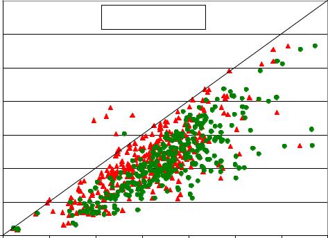
The difference between dynamic and static Young’s Modulus estimates is significantly larger than that observed for Poisson’s Ratio. The data in Figure 9 show static and dynamic Young’s Modulus measurements on the tight-gas and shalegas sample data set measured under “as received” saturation conditions. In all cases, the apparent static modulus is lower than

12	SPE 118703

the dynamic modulus for both high and low axial stress states. Various models have been proposed to correlate dynamic modulus to a more representative static modulus. Each of the proposed models is based on a specific core data set and implied rock type and may not be generally applicable to all rock types. The data sets used here are presented to develop useful correlations specifically for tight-gas and shale-gas reservoirs.

Static Young's Modulus, MMpsi

14.000

Low Axial Stress Dyn E

High Axial Stress Dyn E

12.000

10.000

8.000

6.000

4.000

2.000

0.000
0.000	2.000	4.000	6.000	8.000	10.000	12.000	14.000

Dynamic Young's Modulus, MMpsi

Figure 9: Comparison of core dynamic and static Young’s Modulus values

Eissa and Kazi (1988) are credited with the early work in the area of dynamic to static modulus conversions. They presented two models for well consolidated, low porosity samples. The first model proposed a linear scaling relationship given by Equation 13, while the second model proposed a log linear relationship using the product of core bulk density (ρ, in gm/cm3) and dynamic modulus (Equation 14). In both the Eissa and Kazi models, the dynamic modulus is given in GPa (approximately 6.895 times modulus in million psi).

Es =0.74Ed −0.82	(13)
Log Es =0.02 +0.71Log(ρEd )	(14)
Log Es =Log(ρEd )−0.55	(15)

The proposed models (Equations 13 and 14) were applied to the tight-gas and shale-gas data sets. To obtain the best fit with the current data set the coefficients of Equation 14 were adjusted to those given by Equation 15. The coefficients for Equation 13 were found to give a best-fit straight line for the current data. In addition to the modified Eissa-Kazi models, a power law fit of the form suggested by van Heerden (1987) was also tested. The best-fit power-law model is given by Equation 16.

Es =0.1832Ed1.5795

(16)

Figure 10 shows the static Young’s Modulus values for the entire data set computed from the input dynamic modulus. Of the three equations tested, the modified E-K Log-Linear model (Equation 15) gives the best results by far over the entire range of moduli tested. It is possible that some of the data scatter is reduced by using measured core bulk density measurements made under the same saturation conditions as the corresponding dynamic moduli. While saturation state strongly affects the dynamic Young’s Modulus, the effects of partial saturation on static modulus are not yet known, but are expected to be minor.

SPE 118703	13

	14.000
		Eissa-Kazi Linear
MMpsi	12.000	Power-Law Model
		Modified E-K Log-Linear
Modulus,	10.000
	8.000
Young's
	6.000
Static
Measured	4.000
	2.000
	0.000
	0	2	4	6	8	10	12	14

Computed Static Young's Modulus, MMpsi

Figure 10: Conversion of core dynamic to static Young’s Modulus

Stress and Material Anisotropy

At least two different types of anisotropy must be considered in applying laboratory core data to the calibration of field log data: stress anisotropy and material anisotropy. Many unconventional reservoirs exhibit large-scale inhomogeneity and intrinsic anisotropy including bedding planes, pre-existing fractures, stylolites, and secondary porosity. Large-scale anisotropy and inhomogeneity can significantly affect the apparent mechanical properties (Schatz, 1993). Cicotti and Mulargia (2004) indicate that these large-scale effects generate a bigger difference between core-sample measurements and field-scale log measurements than any correction from static to dynamic that is based on frequency or other factors. The volume of rock integrated by a borehole sonic log is inversely proportional to frequency. As a result, most well logs offer an average DTC and DTS value integrated through many rock layers and include the effects of all fractures, partings, and bedding planes in the result. Miskimins (2002 and 2003) reports that log-derived average acoustic velocities fail to show the degree of stratification apparent in whole core samples. Stress profiles derived from these homogenized acoustic logs fail to adequately predict fracture containment when laminations and fractures are present.

Any large-scale average measurements of rock properties through acoustic measurements must suffer from this problem. Typically, derived stress and rock property profiles will be overly smoothed and will miss discrete layer properties and discontinuities that can act as freely sliding shear planes or stress concentrations in tectonically active areas. Until the use of high-resolution borehole image logs for mechanical properties determination from resistivity or sonic data becomes established, and until fracture models can accurately handle discontinuity effects on a millimeter scale, any fracture geometry or stress profile must be considered to be grossly averaged. As a result, fracture height growth and vertical fracture continuity will be overestimated.

Measurement of anisotropic core properties

A relatively recent development is the measurement of core static and dynamic elastic moduli on adjacent core samples oriented vertically, horizontally, and at 45 degrees to the whole core (wellbore) axis. In some cases of locally homogeneous and isotropic media, the results for three adjacent plug samples are reported to be similar. In other cases, differences in moduli of 2 to more than 5 fold have been reported (verbal communication of proprietary data). Aside from the large-scale effects on anisotropy, the stress field used in these oriented core tests and its impact on observed deformation must be considered.

14	SPE 118703

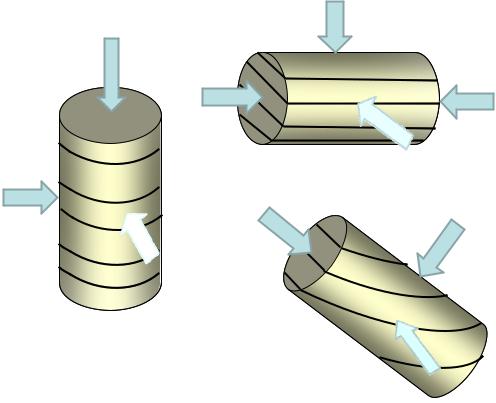
Figure 11 shows a simplified drawing of the three core sample orientations for a core through a horizontally laminated medium. Sample A in Figure 11 shows a vertical plug with an axial load representing the vertical net overburden stress. Lateral deformation is driven by the axial compression normal to bedding. Loading in this orientation appears to derive the appropriate Poisson’s Ratio for use in the modified uniaxial strain equation for horizontal stress estimation (Equation 1). Bilateral anisotropy due to microfractures and grain orientation effects will still cause unequal lateral strains that can be averaged through radial strain measurement.

σz=σv	σr≠σv
	σz=σh
σr=σh	B σr≠σH
	σz≠σv
	σr≠σH
	σr≠σH
A	Optimum angle for
	shear along

	horizontal bedding	C
	σr≠σh
	Figure 11: Diagram of oriented core test loading geometry

Analysis of axial compression of a horizontal core plug parallel to bedding (B) is more problematic. In this case, the applied axial load more closely represents a maximum horizontal stress, as in a thrust-fault environment. The geometry is proposed to represent displacement of the fracture surface by fracturing fluid pressure. Here, the uniform radial confining stress must represent both the vertical stress and the second horizontal stress, which will normally be far from equal in field conditions. For a normal stress state, the radial stress normal to bedding in this laboratory geometry will be far less than the vertical net stress. This can lead to enhanced shear failure along bedding. A potentially more serious concern exists if the sample is not homogeneous. Any bedding layers of high modulus will concentrate load and can give a higher than normal modulus, as compared to an integrated average value. If stress concentration reaches the shear failure limit, the local hard streaks may fail before the softer surrounding rock, leading to odd mechanical behavior. In dynamic measurements, firstarrival acoustic signals will be channeled through the hard streaks, altering interpretations of dynamic properties.

In the case of the 45-degree core orientation (C), the relative angle between the core plug axis and bedding may control failure and apparent moduli. In the orientation shown, the tendency for shear failure along the (potentially) weak bedding planes is maximized. All these core measurements will show differences in acoustic velocity and apparent static or dynamic moduli depending on orientation for locally heterogeneous samples. The difficulty lies in applying these measurements to field predictions of moduli and stress. In most instances, the only wellbore acoustic wave velocities that can be measured will be vertical, and they will correspond most closely to the orientation of sample A in Figure 11. The large-scale measurements will inherently be affected by heterogeneities not captured in intact core plug samples. Overall, the measurement of core properties at different orientations may provide additional information about rock heterogeneity, but these measurements offer no solution to the problem of predicting fracture geometry or closure stress profile.

Acoustic anisotropy

Acoustic anisotropy can be divided into two main categories: vertical velocity anisotropy and vertical to horizontal anisotropy. The use of vertically polarized dipole sonic logs has become common in recent years. In theory, a fast and slow shear wave velocity can be determined from an orthogonally polarized transmitter-receiver pair. Variations in shear velocity

SPE 118703	15

are theoretically related to changes in stress, but can also be caused by changes in saturation, bedding features, fractures, and other environmental factors. Differentiating vertical to horizontal anisotropy seeks to address the tendency of formations to fail in horizontal or low-angle planes (as in delamination or disking of cores). Currently, however, no acoustic borehole logging tools can actually measure horizontal compressional and shear velocities. Vertical to horizontal anisotropy appears to be interpreted based on reflected and refracted tube and surface waves. If properly interpreted, a high degree of vertical to horizontal anisotropy should correlate to better fracture height containment and possibly higher treating pressures.

Brittle-Ductile Characterization of Shale

Shale “reservoirs” have been characterized as brittle versus ductile based on log-derived mechanical properties. More brittle systems are perceived to be easier to fracture while ductile systems deform more plastically and may be more difficult to treat. The degree of brittleness may also relate to the tendency for generation of complex shear fractures. Brittleness, as explained by Mullen et al (2008), is based on apparent Young’s Modulus (E) and Poisson’s Ratio (ν). A formation with low E and high ν is considered ductile, while high E and low ν indicates a brittle formation. The characterization is generally useful for qualitative evaluation of expected treating conditions. Mullen (2008) suggests different fracture treatment designs for varying degrees of brittleness, with the intent of creating complex shear-enhanced fracture networks in britte rocks and planar, high conductivity, fractures in ductile rocks.

It must be remembered, however, that the apparent dynamic moduli used to define brittleness are based on observed acoustic velocities that are affected by TOC, gas content, fractures, and borehole conditions. Applying raw or uncorrected sonic log data may lead to inappropriate characterizations. For example, a highly fractured and gas charged zone may show slow acoustic velocities and be interpreted as a low modulus, high Poisson’s Ratio formation. Its behavior may more closely be modeled by a shattered brittle rock, in terms of appropriate treatment selection.

Examples of Stress Profiles

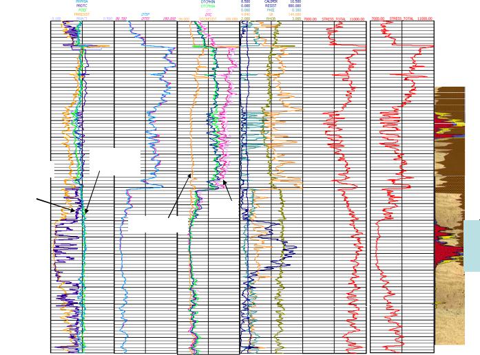
Many of the factors discussed can be illustrated in a field example comparing rock elastic properties and resulting stress profile with actual fracture containment shown by tracer surveys. The log data in Figure 12 cover a range of lithologies. Two separate fracture treatments, indicated by the blue boxes at right, were conducted in the well. The far-left track shows five interpretations of Poisson’s Ratio derived from log values. The green curve (POIS) is the reported dynamic value of ν from a full-waveform dipole sonic log as interpreted by the logging company after complete processing of the data. The blue-gray curve (PRACT) is the value of ν computed using Equations 2 and 4 with no correction for saturation or borehole conditions. The PRACT curve is a direct overlay of POIS over the logged interval, indicating that (as usual) no fluid substitution or other corrections have been applied during “log mechanical properties processing” by the logging company.

The PRPHIA curve in Figure 12 was derived from the crossplot average porosity without use of the measured DTC or DTS data and gives a near perfect overlay of POIS, as is usual. Inputs to this estimate of ν include the estimated matrix and fluid sonic transit times and the neutron-density crossplot porosity. The two dissenting curves, PRDTC and PRRESIST, are derived from compressional sonic travel time and the interpretation of lithology and from deep resistivity independent of lithology and sonic data respectively. In most unconventional reservoirs, these values give the best prediction of stress profile and fracture geometry.

16	SPE 118703
Stress DTS/DTC	Stress PR_RESIST

POIS and

PRRESIST PRACT

PRDTC

DTC

DTCRESIST

Figure 12: Comparison of stress profiles for different log interpretations

The curves in the second track are the reported fast and slow shear slowness reported from the crossed-dipole shear log. A maximum shear anisotropy of 3 μs/ft out of 150 μs/ft (2%) is observed in a few spots over the logged interval, while most of the log shows no discernable shear velocity anisotropy. It is interesting to note that this area is highly faulted and has a known dominant fracture orientation with significant stress anisotropy. It could be that the rock is hard enough that a change in horizontal stress of more than 500 psi has no measurable effect on shear velocity. Other local factors (saturation, organics, and fractures) may have larger impacts. Two stress profiles are presented in Figure 12, computed using the log-derived mechanical properties and Equation 1. The resulting stress profiles are compared to the radioactive tracer log acquired after the fracture stimulation treatments. The stress profile derived from the acoustic DTS/DTC ratio fails to predict the contained fracture observed in the lower perforation set. In contrast, the confined fracture is predicted by the resistivity derived stress profile. In this case both stress profiles would predict a contained fracture geometry for the upper treatment but the magnitudes of the predicted stresses differ by nearly 1000 psi. In most cases the properties derived from sonic velocity measurements fail to give useful predictions of fracture geometry or treating pressure.

Conclusions

Estimation of in-situ stress profiles in unconventional reservoirs is complicated by many factors. Determining pore pressure when matrix permeability is vanishingly small can be nearly impossible by conventional means such as wellbore measurements or even pressure transient tests. Pore pressure can vary locally and to a large degree when driven by hydrocarbon maturation. The local pore pressure is a primary driver of the total closure stress. Pore pressure also affects the net effective stress in the system and can alter acoustic velocities and apparent dynamic moduli.

Acoustic velocities from sonic logs, and dynamic moduli derived from them, can be affected by gas saturation and TOC in tight formations and shale where near-wellbore flushing while drilling is ineffective. The rock volume interrogated and integrated by the sonic log may be at a highly variable saturation state, and the measured sonic velocity may respond more to changes in saturation than to stress or rock property variations. Fractures, laminations, and averaging of dissimilar lithology response can also affect velocity and dynamic properties derived from borehole sonic logs.

SPE 118703	17

Saturation, stress history, anelastic strain, and many other factors also affect core samples used for both static and dynamic measurements of elastic moduli. Core data can be used with care to develop models for deformation and correlation to dynamic properties. Stress cycling and proper saturation of cores is important in deriving useful data for both static and dynamic core measurements. Core samples typically represent point values of intact rock and will give indications of higher strength and isotropy than may actually be present in larger scale samples.

Use of core samples at various orientations can provide useful qualitative information about small-scale anisotropy. This information should be extended to large-scale estimates of stress and deformation with extreme caution. Stress and strain boundary conditions in these oriented core laboratory tests may not be appropriate for field application.

Use of synthetic sonic logs and elastic moduli is strongly encouraged in unconventional reservoirs. If the derived data confirms the direct acoustic measurements, then it is possible to derive some degree of comfort. When the synthetic derived data and measured sonic data disagree, there is usually a good and definable reason. If the cause of the discrepancy can be traced to pore fluid, pore pressure, or discontinuity effects, then the synthetic data typically give better and more useful estimates of the necessary rock properties for both stress profile calculation and fracture geometry evolution.

Nomenclature
CEG	:	Constant offset for estimation of E from GR
CER	:	Constant offset for estimation of E from resistivity
CPG	:	Multiplying pre-factor for estimate of ν from GR
DTS	:	Shear sonic slowness, microseconds/ft
DTC	:	Compressional sonic slowness, microseconds/ft
DTC_PHIA	:	Compressional slowness estimated from crossplot average porosity fraction, microseconds/ft
DTFL	:	Pore fluid sonic travel time (slowness), microseconds/ft
DTMA	:	Rock matrix sonic travel time (slowness), microseconds/ft
Ε	:	Young’s Modulus, million psi (unless otherwise specified)
Es	:	Static Young’s Modulus
Ed	:	Dynamic Young’s Modulus
EER	:	Exponent for estimation of E from resistivity
EPG	:	Exponent for estimation of ν from GR
EPR	:	Exponent for estimation of ν from resistivity
GR	:	Total gamma-ray counts, API units
Ish	:	Dimensionless GR index
OEG	:	Constant offset for estimation of E from GR
Pc	:	Total fracture closure stress or minimum in-situ stress, psi
Pp	:	Pore pressure, psi
R	:	Square of sonic travel time ratio, dimensionless
RESIST	:	Formation electrical resistivity, OHMM
Sw	:	Water saturation in pore space, fraction
Vp	:	Compressional acoustic velocity, ft/sec
Vs	:	Shear acoustic velocity, ft/sec
Vsh	:	Volume fraction shale (or clay) in formation
YME_GR	:	E estimated from GR, million psi (unless otherwise specified)
YME_RESIST	:	E estimated from resistivity, million psi (unless otherwise specified)
YME_PHIA	:	E estimated from crossplot average porosity, million psi (unless otherwise specified)
αv	:	Vertical poroelastic constant, dimensionless
αh	:	Horizontal poroelastic constant, dimensionless
εh	:	Horizontal tectonic strain normal to minimum stress, microstrains
ν	:	Poisson’s Ratio, dimensionless
φ	:	Porosity, fraction
ρb	:	Bulk density, g/cm3
σh	:	Minimum horizontal total stress, psi
σt	:	Tectonic stress offset, psi
σv	:	Vertical total overburden stress, psi

18	SPE 118703

References

Al-Shayea, N. A.: “Effects of testing methods and conditions on the elastic properties of limestone rock,” Engineering Geology v. 74, pp. 139–156. 2004.

Blanton, T.L., and Olson, J.E.: “Stress Magnitudes from Logs: Effects of Tectonic Strains and Temperature,” SPE Reservoir Evaluation & Engineering, Volume 2, Number 1, Pages 62-68, February 1999.

Briaud, Jean-Louis, “Intro to Moduli’”, ceprofs.tamu.edu/briaud/, 2008.

Ciccotti, M. and Mulargia, F.: “Differences between Static and Dynamic Elastic Moduli of a Typical Seismogenic Rock,” Geophys. J. Intl., v. 157, pp. 474-477, 2004.

Crain, E. R., CRAIN'S PETROPHYSICAL HANDBOOK, http://www.spec2000.net/chapters/Chapter06.htm, Rocky Mountain House, Alberta, Canada, 2008.

Eissa, A., Kazi, A.: “Relation between static and dynamic Young’s moduli of rocks,” Int. J. Rock Mech. Min. Sci. Geomech. Abstr. Volume 25, Number 6, Pages 479– 482, 1988.

Holmes, M., Holmes, A., and Holmes, D.: “Modification of the Wyllie Time Series Acoustic Equation, to Give a Rigorous Solution in the Presence of Gas,” presented at the SPWLA 45th Annual Logging Symposium, Noordwijk, The Netherlands, June 6-9, 2004.

http://Hyperphysics.phy-astr.gsu.edu/hbase/sound/souspe3.html, 2008. http://server4.oersted.dtu.dk/research/RI/SNG/SNG-logs.html, 2008.

Knight, R., Dvorkin, J. and Nur, A.: “Acoustic Signatures of Partial Saturation,” GEOPHYSICS, v. 63, n. 1, pp. 132–138, Jan-Feb 1998. La Gesse, J., and Hurley, N.: “Predicting Source Rock Quality using GR Wireline Response and Umaa vs. ρmaa Crossplots in the Lewis

Shale, Green River Basin, Wyoming,” paper SPE 114963 presented at the 2008 SPE Annual Technical Conference and Exhibition, Denver, Colorado, U.S.A., 21-24 September 2008.

Li, Yongyi and Schmitt, D. R.: “Well-Bore Bottom Stress Concentration and Induced Core Fractures,” AAPG Bulletin, V. 81, No. 11 P. 1909–1925, November 1997.

Lim, S. S., Martin, C. D., and Christiansson, R.: “Estimating In-Situ Stress Magnitudes from Core Disking,” In-Situ Rock Stress – Lu, Li, Kjerholt, and Dahle (eds), Taylor and Francis Group, London, ISBN 0-415-40163-1, 2006.

Merkel R. H. and Barree, R. D., and Towle, G.: “Seismic Response of Gulf of Mexico Reservoir Rocks with Variations in Pressure and Water Saturation,” THE LEADING EDGE, pp. 290-299, March 2001.

Miskimins, J. L. and Barree, R. D.: “Modeling of Fracture Height Containment in Laminated Sand and Shale Sequences,” paper SPE 80935 presented at the Production and Operations Symposium held in Oklahoma City, OK, March 22-25 2003.

Miskimins, J. L., Hurley, N., and Graves, R.: “A Method for Developing Rock Mechanical Property Logs using Electrofacies and Core Data,” paper SPE 77783 presented at the SPE Annual Technical Conference and Exhibition, San Antonio, TX, Sept 29-Oct 2, 2002.

Morales, R. H. and Marcinew, R. P.: “Fracturing of High Permeability Formation: Mechanical Properties Correlations,” paper SPE 26561 presented at the 68th Annual Technical Conference and Exhibition, Houston, TX, October 3-6, 1993.

Mullen, M., Russel Roundtree, R, Barree, R.: “A Composite Determination of Mechanical Rock Properties for Stimulation Design (What to do When You Don’t Have a Sonic Log),” paper SPE 108139 presented at the 2007 SPE Rocky Mountain Oil & Gas Technology Symposium, Denver, Colorado, U.S.A., 16–18 April 2007.

Passey, Q. R., Creaney, S., Kulla, J. B., Moretti, F. J., Stroud, J. D.: "A Practical Model for Organic Richness from Porosity and Resistivity Logs", AAPG Bull., Dec. 1990.

Perreau, P.J., Heugas, O., and Santarelli, F.J.: “Tests of ASR, DSCA, and Core Disking Analyses to Evaluate In-Situ Stresses,” paper number 17960 presented at the Middle East Oil Show, March 11-14, 1989, Bahrain.

Rickman, R., Mullen, M., Petre, E,, Grieser, B., Kundert, P.: “A Practical Use of Shale Petrophysical Properties for Stimulation Design Optimization: All Shale Plays are not Clones of the Barnett Shale,” paper SPE 115258 presented at the 2008 SPE Annual Technical Conference and Exhibition, Denver, Colorado, U.S.A., 21-24 September 2008.

Rondeel, H.E.: “HYDROCARBONS,” Tekst voor de cursus Grondstoffen en het Systeem Aarde (HD 698), pp. 17-30 December 2001. Schatz, J. F., Olszewski, A. J., and Schraufnagel, R. A.: “Scale Dependence of Mechanical Properties: Application to the Oil and Gas

Industry,” paper SPE 25904 presented at the SPE Rocky Mountain Region/Low Permeability Reservoirs Symposium, Denver, CO, April 12-14, 1993.

Stieber, S. J., and Thomas, E. C.: “The Distribution of Shale in Sandstones and its Effect upon Porosity,” SPWLA Sixteenth Annual Logging Symposium, June 4-7, 1975.

Thiercelin, M. J., and Plumb, R. A.: “Core-Based Prediction of Lithologic Stress Contrasts in East Texas Formations,” SPE Formation Evaluation, pages 251-258, Dec. 1994.

Van Heerden, W.L.: “General relations between static and dynamic moduli of rocks,” Int. J. Rock Mech. Min. Sci. Geomech. Abstr. Volume 24, Number 6, Pages 381– 385, 1987.

Warpinski, N.R., Peterson, R.E., Branagan, P.T., Engler, B.P., and Wolhart, S.L.: “In Situ Stress and Moduli: Comparison of Values Derived from Multiple Techniques,” paper SPE 49190 presented at the 1998 SPE Annual Technical Conference and Exhibition held in New Orleans, Louisiana, 27-30 September 1998.

Warpinski, N.R., Teufel, L.W.: “A Viscoelastic Constitutive Model for Determining In-Situ Stress Magnitudes From Anelastic Strain Recovery of Core (includes associated papers 19042 and 19892 ),” Journal SPE Production Engineering, Volume 4, Number 3, Pages 272-280, August 1989.

Yassir, N., Wang, D. F., Enever, J.R., and Davies, P.J.: “Experimental Analysis of Anelastic Strain Recovery of Synthetic Sandstone Subjected to Polyaxial Stress,” Paper 47238 presented at the SPE/ISRM Rock Mechanics in Petroleum Engineering, Trondheim, Norway, July 8-10, 1998.