SPE-118703-MS

SPE 118703

Stress and Rock Property Profiling for Unconventional Reservoir Stimulation

R.D. Barree and J.V. Gilbert, Barree & Associates LLC, and M.W. Conway, Stim-Lab, Inc.

Copyright 2009, Society of Petroleum Engineers

This paper was prepared for presentation at the 2009 SPE Hydraulic Fracturing Technology Conference held in The Woodlands, Texas, USA, 19–21 January 2009.

This paper was selected for presentation by an SPE program committee following review of information contained in an abstract submitted by the author(s). Contents of the paper have not been reviewed by the Society of Petroleum Engineers and are subject to correction by the author(s). The material does not necessarily reflect any position of the Society of Petroleum Engineers, its officers, or members. Electronic reproduction, distribution, or storage of any part of this paper without the written consent of the Society of Petroleum Engineers is prohibited. Permission to reproduce in print is restricted to an abstract of not more than 300 words; illustrations may not be copied. The abstract must contain conspicuous acknowledgment of SPE copyright.

Abstract

Sonic log data and core measurements are often used to develop models of in-situ stress profiles and rock elastic properties for use in hydraulic fracture design treatments in unconventional reservoirs. “Unconventional” reservoirs, for the purposes of this paper, include shale-gas, coalbed methane, and tight-gas projects. In unconventional reservoirs, many of the assumptions underlying rock property estimation and stress profiling in conventional reservoirs may not apply. In fact, the result of using conventional approaches may be an incorrect and often misleading stress profile. Fracture geometry predicted using conventionally derived rock properties and stresses might also be inaccurate.

Methods of deriving rock properties from log and core measurements and the effect of various parameters on resulting moduli and stress estimates are examined. The paper also discusses the effects of rock anisotropy and inhomogeneity on static and dynamic properties. The impact of organic materials and trapped gas on sonic logs and conventional mechanical properties interpretation and the use of synthetic sonic logs are also presented. For static and dynamic measurements on core samples, the effects of the condition of recovered core and applied laboratory procedures on measurement results are also considered.

Potential errors resulting from the use of inappropriate mechanical properties for stress profiling and fracture geometry prediction can be significant. The paper identifies common pitfalls in core and log interpretation. A recommended procedure to determine useful and accurate rock mechanical properties for stress profile prediction and fracture design is presented.

Introduction

Full-waveform sonic logs and core measurements are commonly used to derive “calibrated” models of in-situ stress profiles. The results are used as input to hydraulic fracture design simulators, which are used to determine optimum perforation placement, job size, pump rate, fluid and proppant requirements, and other design variables for optimum reserve recovery. The methods used to determine rock mechanical properties and stresses assume that the raw input measurements are valid and that the conditions of measurement are appropriate to conditions during hydraulic fracturing. In unconventional reservoirs, these assumptions may not be valid.

Because of the potential for large reserves, there is an increasing interest in unconventional reservoirs. For the purpose of this discussion, unconventional reservoirs are considered to be tight and ultra-tight gas sands (less than 0.01 md effective permeability), gas-shales, and coalbed methane (CBM) reservoirs. These reservoirs have several characteristics in common: They all have low, very low, or nearly immeasurable “matrix” permeability. They may be self-sourcing and can contain organic carbon within the hydrocarbon maturation window, and may be actively generating hydrocarbons at the time of discovery and development. Many have abnormal pore pressures, relative to a hydrostatic gradient. Many occur in regions with significant tectonic stress or strain overprints, hence anisotropic stress fields. Production from these reservoirs is commonly enhanced through the presence of some kind of fracture or micro-fracture network.

These complexities affect the behavior of core and log measurements. Interpretation of core and log data may require different paradigms and assumptions than those commonly applied in more conventional reservoir systems. Using conventional assumptions when dealing with measurements in unconventional reservoirs can lead to significant errors in the derived rock mechanical properties and estimated stress profile. These errors can lead to incorrect predictions of fracture containment and overall geometry, conductivity, and post-frac performance.

Estimation of In-Situ Minimum Horizontal Stress

The hydraulic fracture closure pressure is assumed to represent the minimum of the three principal stresses acting on the rock affected by the fracture. In conventional reservoirs at moderate depths, the minimum stress is typically assumed to be

2	SPE 118703

horizontal and to follow some form of the uniaxial strain model. Equation 1 gives a slightly expanded form of the uniaxial strain estimate of minimum horizontal stress.

P =σ

=

ν

[σ

−α

P ]+α

P +ε

E +σ

(1)

(1−ν)

c

h

v

v p

h p

h

t

The observed fracture closure pressure (Pc) is assumed to equal the minimum horizontal stress (σh) in this model. The magnitude of σh is assumed to be controlled by the vertical uniaxial strain with externally applied horizontal tectonic stress and strain offsets. As discussed by Thiercelin (1994), the model is very simplistic considering the complex deposition, diagenetic, and deformational history of most reservoir systems. Warpinski (1998) suggests that the two poroelastic constants (αv and αh) are equal for isotropic materials. This is incorrect and misinterprets the physical meaning of the pore pressure terms in Equation 1. The first term in brackets, involving αv, is the vertical net effective stress causing compaction of the rock framework. In this term, the internal pore pressure acts against the externally applied overburden stress to reduce net intergranular stress. The pore pressure term must be corrected for cementation, consolidation, and other poroelasticity effects. The second pore pressure term, involving αh, does not involved net intergranular stress but refers to internal fluid pressure only. The pore pressure acts equally in all directions and is in direct hydraulic communication with the fracturing fluid. In this case, no poroelastic effect should be applied, and the αh term should be set to unity or removed from the equation.

The observed minimum stress commonly differs from that calculated from the uniaxial strain assumption. The differences may be caused by errors in estimation of elastic properties (α, ν and E), pore pressure, and overburden stress, or through externally applied horizontal stresses and strains. In Equation 1, only stresses and strains normal to the plane of minimum stress are considered, although transverse stresses may be generated through other applied strains. Since stresses and strains other than the minimum cannot be resolved, they will not be considered in detail here. The maximum stress induced by an applied lateral strain (ε) is limited by the shear failure envelope of the material, as discussed by Thiercelin (1994). Accurate determination of the shear limit requires knowledge of the complete in-situ net stress tensor and rock strength (in shear) along the potential plane of weakness. Typically, none of these can be determined from field data. Instead, a practical maximum strain limit can be set for use in calibrating stress profiles. The practical limit can be derived from an assumed material cohesion and friction angle along with an estimate of vertical net effective stress. Using the applied strain boundary condition has been shown to give more accurate derived stress profiles than a constant stress offset (Blanton, 1999). The stress offset may be useful to describe residual background stress after inset of shear failure in an active fault environment.

Application of Equation 1 requires representative values of rock mechanical properties. Values of Young’s Modulus (E) and Poisson’s Ratio (ν) can be determined from core samples (both static and dynamic acoustic tests) and from well log (dynamic acoustic) measurements. The accuracy and applicability of these derived properties has a direct impact on the calculated stress profile, even when it is “calibrated” to a single point of measured closure stress. When rock properties and environmental or test conditions affect the apparent mechanical properties, errors in stress and fracture geometry can result. Unconventional reservoirs offer many opportunities for these errors to occur. In addition, Equation 1 implies that the stress profile affecting fracture propagation and geometry is the result of an equilibrium deformation state for an elastic medium. Unconventional reservoirs, especially coal and shale, may behave as ductile or plastic materials rather than elastic ones. During hydraulic fracturing, the rock must respond to rapidly induced deformation. In very low permeability systems, a rapid strain rate can outrun the ability to dissipate internal pore pressure. This can result in deformation behavior controlled by “undrained” moduli instead of “drained” moduli. Many more complex factors must be considered in deriving a stress profile and fracture geometry in these complex reservoirs.

Use of Sonic Transit Time for Mechanical Properties

Full-waveform sonic logs, yielding both shear and compressional wave travel time (DTS and DTC respectively) are commonly used to derive dynamic elastic properties. The assumption is that the acoustic velocities are related to the rock elastic properties. Conventional equations for Poisson’s Ratio (ν) and Young’s Modulus (E) are given as Equations 2 and 3:

	ν =	(R −2)				(2)
		(2R −2)
	E =13447ρb		(3R −4)			(3)
			(DTC 2 R(R −1))

In these equations, the observed formation bulk density (in g/cm3) is given by ρb, and R is the square of the travel-time ratio:

	R =	DTS 2	(4)
		DTC 2

SPE 118703	3

The travel times (DTC and DTS) are the reciprocals of the compressional and shear acoustic wave velocities (Vp and Vs) respectively. Equations 2-4 are equivalent to the dynamic moduli definitions of Lama and Vutukuri as cited by Warpinski (1998). The mechanical properties derived from sonic measurements are assumed to correlate to “static” measurements made on core samples. Unfortunately, things other than variations in elastic rock properties significantly affect the sonic velocities. These other factors include fractures and laminations, external stress, temperature, borehole conditions (breakouts, mud weight, borehole size, and tool eccentricity), pore pressure, and pore fluid saturation. In many cases, there is no correction or adjustment made to the observed sonic transit times for any of these effects.

Error Propagation in Dynamic Moduli Calculation

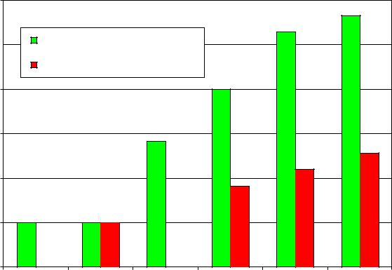
Compressional and shear sonic velocities are intrinsically difficult to measure due to the nature of the wave train and the borehole environment. Various methods are used to reduce the error in detecting and measuring the compressional and shear arrivals, such as Slowness Time Coherence (STC) plots. The inherent noise in the system, however, makes eliminating all error impossible. The equations above are used to calculate the dynamic Poisson’s Ratio and Young’s Modulus from the shear and compressional arrivals. The reliance of these forms on R (equation 4), the ratio of the shear slowness squared over the compressional slowness squared, leads to large errors being propagated through to the mechanical properties. An analysis has been performed considering a +/- 5% error in both the shear and the compressional velocity measurements, shown by the first two bars in Figure 1, to show how that error propagates through into the dynamic Young’s Modulus and Poisson’s Ratio calculations. Assuming that the density measurement is error free, the Poisson’s Ratio has an inherent error of +/- 20% and the Young’s Modulus has a final error of +/- 26%. When calculating stress, the ratio of Poisson’s Ratio to one minus Poisson’s Ratio is used, increasing the error to +/- 28%. Figure 1 summarizes the error analysis.

	30.0%
	25.0%	Properties from DTS/DTC
		Properties from DTCO and Lithology
- %	20.0%
+/
Analysis	15.0%
Error	10.0%
	5.0%
	0.0%
		DTSM	DTCO	R	PR	YME	PR/(1-PR)

Figure 1: Propagation of errors with a 5% error in sonic velocities

Errors of this magnitude obviously have a large effect on the final stress profile calculated using these mechanical properties. Calculating the same mechanical properties using a correlation based on compressional velocity alone (no shear input) leads to a reduction in the potential error. Dynamic Young’s Modulus can easily be obtained using compressional velocity only. Figure 2 shows a regression through 327 tight-gas and shale-gas core samples that gives an excellent estimate of the dynamic modulus measured under controlled laboratory conditions. Using a lithology volume fraction weighted average value of ν (based on the curves presented in Mullen, 2008) can give a good estimate of Poisson's Ratio. For a

4	SPE 118703

sand/shale lithology with an assumed +/- 5% error in the compressional velocity, the Poisson’s Ratio error is 9%, with a total error of 11% for the Young’s Modulus (if the correct shale fraction is known). The error in the ν/(1-ν) term is 14%, or half the error resulting from using both the shear and compressional velocities in equation 4.

18
16
14	y = 54857x-2.1557
	R2 = 0.9665

12

10

8

6

4

2

0

40

60

80

100

120

140

160

Vp Transit Time, micro-sec/ft

Figure 2: Estimation of dynamic Young’s Modulus from Vp alone

Generating a stress profile based on the shear/compressional ratio results in the magnification of any inherent errors in the measurements of both shear and compressional wave slowness. Both the shear and compressional slowness values from acoustic borehole logs can be subject to significant error of measurement and interpretation. Using a diagnostic injection test to measure minimum in-situ stress can help to ensure the validity of the calculated stress profile. Using a correlation not based on shear velocity, and correcting compressional velocity data for saturation and environmental effects also results in less error prone mechanical properties.

Effect of Gas Saturation on Sonic Logs and Stress Estimates

The impact of hydrocarbon saturation on sonic velocity has been studied extensively (Merkel, 2001 and Holmes, 2004). Holmes (2004) shows that the presence of 20% gas saturation can change the observed compressional travel-time for a sandstone reservoir by 25% compared to a water saturated sample. Using measured water velocity data from Merkel (2001) and calculated gas acoustic velocity (hyperphysics.phy-astr.gsu.edu/hbase/sound/souspe3.html), the volume average DTC can be estimated using the Wyllie Time Series Acoustic Equation (Homes, 2004) given here as Equation 5:

DTC =φDTFL +(1−φ)DTMA

(5)

In Equation 5, DTFL is the volume-average fluid acoustic velocity for a gas-water mixture and DTMA is the matrix transit time. Figure 3 shows the computed change in apparent Poisson’s Ratio (ν) using an assumed DTC at 100% Sw of 64.5 μs/ft (DTMA=53 μs/ft and DTFL=197 μs/ft) and a constant DTS of 126 μs/ft. The assumption of constant DTS is based on the (probably incorrect) belief that the acoustic shear wave is transmitted only through the solid matrix and is unaffected by pore fluid. A change in gas saturation from 0% to 60% causes ν to drop from 0.32 to 0.03 for these assumptions. This magnitude of change is greater than the typical contrast between clean sand and plastic shale, and it drastically affects the estimated stress profile. Laboratory measurements of sonic velocity in water at various pressures, and in oil at and below the saturation pressure (Merkel, 2001), show that velocity changes of this magnitude can occur in gas-water systems and in water-oil systems. In oil reservoirs, the acoustic velocity changes dramatically at the saturation pressure when free gas is generated. Similar effects can be expected in organic rich shale in the gas generation (maturation) window.

SPE 118703	5

	0.35
	0.3
Ratio	0.25
Poisson's	0.2
	0.15
Apparent
	0.1
	0.05
	0
	0	0.1	0.2	0.3	0.4	0.5	0.6	0.7

Gas Saturation

Figure 3: Effect of gas saturation on Poisson’s Ratio for variable DTC with constant DTS

Use of Spectral GR Logs to determine TOC and Vshale

In conventional reservoirs, the producing interval is generally a “clean” sand or carbonate surrounded by “shale”. The shale bounding beds are considered to be non-reservoir rocks and are commonly expected to provide some degree of fracture height containment. The volume-fraction “shale” is often computed from a normalized total gamma ray (GR) log using one of several published relations (Crain, 2008), such as Steiber’s correlation (Steiber, 1975), given as Equation 6:

	Vsh =	0.5I sh		(6)
		(1.5	− I sh )

In Equation 6, the GR Index (Ish) is the normalized value of the selected GR curve between the value of GR at the apparent “clean sand” line (GRsand) and at the “100% Shale” line (GRshale), as shown by Equation 7:

	Ish =	(GR −GRsand )	(7)
		(GRshale −GRsand )

The total GR observed response is generated by many species of radioactive material in the rock. A spectral GR tool differentiates three principal components: thorium, potassium, and uranium. Of these components, thorium is generally associated primarily with clay minerals. Potassium may be associated with clays, potassium-feldspars, salts, and other materials that may be rock constituents. Uranium is most often associated with organic matter and precipitated salts and is generally not related to clay content. Uranium response can often be correlated to total organic carbon (Crain, 2008, La Gesse, 2008), while clay content can be more accurately related to thorium, and possibly potassium, content.

Unconventional reservoirs may contain relatively large amounts of total organic carbon (TOC), and may be hydrocarbon source-rocks (especially shales). It is common to find a high total GR response in organic-rich shale while actual clay content may be only 3 to 20%. Basing the shale volume-fraction (Vshale) estimate on normalized total GR can imply that hydrocarbon rich, high TOC zones are non-reservoir when in fact they are the primary completion target. Incorrect Vshale estimates also affect the implied plasticity of the rock and the estimated values of mechanical properties if lithology-based correlations are applied. Besides the impact of organic material on shale or clay content estimates, the presence of organic material can also have a significant impact on acoustic velocity measurements, calculated dynamic rock mechanical properties, and estimated in-situ stress. All these effects are tied to the generation of hydrocarbons (gas and or oil) from solid kerogen in shale source-rocks.

As kerogen matures and generates free hydrocarbons, the volume of the organic material increases dramatically. Because of the small pore size, high capillary threshold pressure, and low permeability of shale, the generated hydrocarbons may remain trapped in the pore system until it reaches a pressure sufficient to generate hydraulic (micro) fractures. For a hydrocarbon sourcing shale in the gas generation window, this can mean that the internal pore pressure can actually reach the

6	SPE 118703

fracture pressure of bounding rocks or of the shale itself (Rondeel, 2001). Some (unreleased) field data confirms pore pressures in shale nearly equal to the fracture closure stress in surrounding layers. Net effective stress within the shale can be very low, even at great depths, making the formation susceptible to shear failure at low differential stress. The presence of gas in the pore space, along with the elevated internal pressure, results in dramatic slowing of the compressional acoustic signal and abnormally high observed values of DTC.

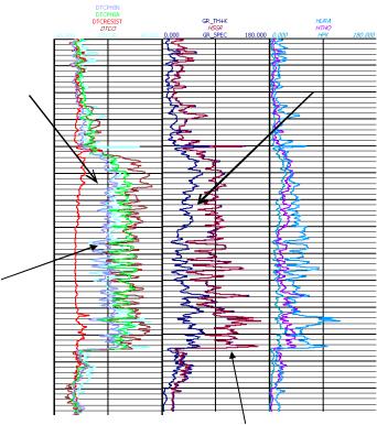
As an example, Figure 4 shows the total high-resolution GR (HSGR) curve and a total GR composed of the sum of the scaled spectral GR input curves (GR_SPEC). The individual spectral GR components are plotted in the far-right track of the figure, after scaling to API units. Scaling is accomplished by multiplying the thorium signal (ppm) by 4.0, uranium (ppm) by 8.0, and potassium volume fraction (v/v) by 1500. These scaling factors have been found to give comparable total GR curves in most cases, although other scaling factors have been published (http://server4.oersted.dtu.dk/research/RI/SNG/SNGlogs.html, 2008). The GR_TH+K curve in Figure 4 is the scaled total GR, without the uranium component. This curve, sometimes referred to as the Computed GR (CGR) gives a better appreciation of actual mineralogy and clay content for the organic rich shale.

The log section at far left in Figure 4 shows the measured and derived (synthetic) DTC curves for the well. The DTCO curve is the measured compressional travel time. It is significantly affected by the organic material and generated gas in the shale. The result is an abnormally slow DTC compared to the synthetic DTC curves that match the measured DTC above and below the gas/TOC zone. Using the anomalous measured DTC curve will generate incorrect estimates of dynamic elastic properties for the rock. Use of a synthetic DTC curve, or DTC corrected for the presence of gas saturation and TOC, may give a better estimate of rock elastic properties. Improved estimates of rock elastic moduli generate more accurate computed stress profiles when elastic deformation is expected. Only careful calibration of the computed stress profile to a directly measured stress allows the best of the many possible DTC interpretations to be selected. Many field cases have been studied in which the measured DTC clearly leads to incorrect stress profiles while synthetic DTC curves give useful results.

		Separation due
Sonic Slowing due
to Gas and TOC		to Uranium in
Effects		Organics

DTC from

Resistivity

DTC from

PHIN and GR

DTC Measured

Measured total GR and GR_SPEC

Figure 4: Effect of organic material on GR and DTC

Derivation of Mechanical Properties from Non-Sonic Logs

The use of derived synthetic compressional sonic logs has been presented by Mullen, et al (2007). Methods are presented to derive DTC curves from simple scaling models applied to computed GR (without organic effects), neutron and crossplot porosity, and deep electrical resistivity (beyond the invaded zone). The methods and models used are an outgrowth of the

SPE 118703	7

Passey (1990) technique, which relates TOC percentage to the sonic and resistivity response. In estimating rock properties, it is advantageous to use the same response to eliminate the gas and TOC effect.

The synthetic DTC curves in Figure 4 were derived using models similar to those presented by Mullen (2007) and calibrated to the local log conditions in zones expected to be at 100% Sw. Local calibration or scaling of the derived DTC curves is recommended to detect small variances in the measured DTC that can show trapped gas in the region investigated by the sonic tool. In organic-rich shale formations, the effect on the measured sonic is typically large, as in the case shown.

The relative magnitudes of the derived and measured DTC curves are systematic and diagnostic. In formations with high gas or TOC content, the measured DTC will be slowest. The DTC computed from average total porosity (neutron-density crossplot porosity) will generally be very close to the measured DTC curve as both neutron and density response will be affected by gas and TOC. The DTC curves derived only from neutron porosity will give the next lower values of DTC, and DTC from deep resistivity will give the fastest estimate of transit time slowness. In developing synthetic rock mechanical properties and stress profiles, use of the DTC from resistivity often gives the best correlation to observed closure stress and fracture height development.

Elastic moduli (ν and E) can be derived from the synthetic DTC curves using lithology volume fractions, as demonstrated by Mullen (2007). These moduli can also be derived directly from conventional open-hole log responses using simple models. For example, useful estimates of Poisson’s Ratio can be derived using power-law functions of resistivity and computed GR, as shown by Equations 8 and 9:

PR_GR=CPG*GREPG	(8)
PR_RESIST=CPR*RESISTEPR	(9)

The coefficients in Equations 8 and 9 are obtained by correlation of the derived synthetic curves to values of ν computed from DTC and lithology, or travel-time ratio (R), in areas of good borehole condition and 100% water saturation (usually non-reservoir intervals). Similarly, good estimates of E can be derived directly from open-hole log responses using simple linear scaling, power-law, and exponential equations, as shown in Equations 10-12:

YME_GR=CEG*GR+OEG	(10)
YME_RESIST=CER*RESISTEER	(11)
YME_PHIA =62*10(-0.0145*DTC_PHIA)	(12)

Other useful estimates of mechanical properties can be derived from various combinations of log measurements, including cased-hole pulsed neutron logs. The key is that dynamic properties derived from measured full-waveform acoustic logs can be used to develop correlations when the data from the sonic logs are valid. This is only the case in 100% watersaturated rocks with good borehole conditions and intact rock with minimal open fractures. Even then, the pore pressure must be nearly constant across the zone used for calibration. As shown by Merkel, et al (2001) both shear and compressional velocity vary with net stress to the 1/3 power. If pore pressure changes locally, especially in a hydrocarbon sourcing shale, then all observed velocities will be poor representations of rock elastic properties. Elastic properties computed from uncorrected (measured) sonic-derived properties will be wrong, and the estimated stress profile will be incorrect due to both erroneous elastic moduli and incorrect pore pressure assumptions.

Use of Unconventional Core Mechanical Properties Data

Many people believe that static core measurements of elastic moduli represent a “ground-truth” for calibration of dynamic core properties or log-derived dynamic moduli. Unfortunately, in unconventional reservoirs, there are many processes associated with core recovery, transport, and processing that can make the core that is studied in the laboratory less than ideal as a representation of in-situ rock properties.

In the reservoir, the core is at stable internal pore pressure and temperature, and supported by anisotropic confining stresses. During drilling and coring, the overburden stress is released and replaced by the circulating mud weight. Lateral stresses acting on the rock below the bit face can generate sufficient stress concentrations to cause core disking and other shear and tensile fracture modes (Li, 1997, Lim, 2006). As the core bit passes the sample, lateral stresses are released allowing lateral expansion and possible generation or enhancement of fractures to occur. During core recovery, the internal pore pressure is released. For extremely low permeability samples, the release of pore pressure may be accompanied by expulsion fracturing or enhancement of existing fractures. Finally, at the surface the sample may experience thermal contraction, desiccation, and possible oxidation of clay minerals. All these factors can cause mechanical failure, fracture, and changes in elastic properties. The characteristics of unconventional reservoirs will exacerbate these effects.

The impact of micro- (and macro-) facture generation during coring has long been observed. Both anelastic strain recovery (ASR) and differential strain curve (DSC) analysis have been used to determine the orientation and relative magnitude of in-situ stresses. These methods involve the measurement of anisotropic strains resulting from core relaxation

8	SPE 118703

after recovery. In most cases, the observed strains are believed to be caused by opening of fractures normal to the maximum in-situ stress (Warpinski, 1989, Yassir, 1998). These observations make it a near certainty that a core sample from an unconventional reservoir will not represent in-situ stress or mechanical properties without some attempt to restore the sample’s integrity.

Effects of stress and strain relaxation and cycling on static and dynamic moduli

When core samples are subjected to static or dynamic testing in a laboratory, the confining stress, net effective stress, stress history, pore pressure, temperature, and saturation state may all affect the results. Traditionally, core samples are tested in the “as received” condition and the primary compaction cycle is used to derive static moduli. If the core has developed open microfractures during coring and handling, and is partially gas saturated, these measurements may not reflect the expected in-situ conditions. In general, the core will deform more easily because of the increased compliance of the fracture network, giving a Young’s Modulus that is too low to represent deformation during fracturing. Applied axial loads will close fractures and generate less lateral strain than would be the case for an intact sample, leading to abnormally low Poisson’s Ratio. The absolute magnitude and differential stress state established at the start of the test also has a significant effect on the observed material properties. Often the confining stress is poorly defined.

Stress
DIfferential		E4
	E5
	E2	E3
	E1

Axial Strain

Figure 5: Effect of stress cycling on apparent Young’s Modulus

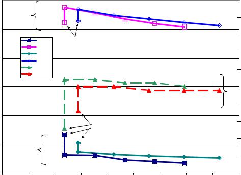
One way to partially offset the effects of core relaxation and microfracture evolution is to stress-cycle the sample before taking measurements of stress and strain to describe moduli for stress profiling or fracture geometry estimates. Figure 5 shows a hypothetical stress-strain profile for a core sample under cyclic loading. Five different Young’s Modulus values are illustrated corresponding to the initial compaction modulus (E1), low net stress tangent modulus (E2), unloading tangent modulus (E3), high net stress tangent modulus (E4), and high net stress secant modulus (E5). As described by Briaud (2008), many other modulus values may be defined, and the proper modulus for use in a particular case must be selected to represent local deformation and stress conditions. In an unconventional reservoir, core E1 is likely to represent a partially failed state with open fractures, and is not representative of conditions during fracturing. Assuming the rock has not been subjected to multiple stress cycles over a short time, the unloading modulus (E3) is not representative. The secant modulus (E5) may be useful to estimate long-term residual deformation after multiple stress cycles, but is not useful for fracture geometry or stress prediction. This leaves the high or low stress tangent moduli E2 and E4.

During hydraulic fracturing, the rock is subjected to fairly rapid deformation, starting at a stable in-situ stress state. If the in-situ stress and strain conditions could be maintained throughout the coring and handling process, then measuring the tangent modulus at the average net effective stress should be the correct conditions (Warpinski, 1998). Because the core must be re-compacted, a better estimate can more often be obtained using a higher net effective stress than that existing in the

SPE 118703	9

reservoir. If a prolonged linear stress-strain regime exists through several stress cycles, the selection of proper stress state is simplified and the overall linear trend can be used. In general, the most useful modulus is that which describes the process being modeled.

Effects of saturation state on static and dynamic moduli

Core acoustic measurements are frequently used to verify and calibrate properties derived from logs. Static mechanical properties measurements are also used to derive conversions from dynamic to static moduli. The effects of saturation and stress on acoustic velocity measurements that are observed in well logs also exist in laboratory core measurements, along with stress cycling effects. Many times these effects are ignored or neglected. In very low permeability systems, it is common practice to perform static deformation studies in an “as received” or unknown saturation state. Even with small gas saturations in core samples, the acoustic velocity of the core-fluid system can change significantly. The saturation may change dramatically with pore pressure and sometimes with external stress, introducing further uncertainty in the measurements. When core and log sonic velocity measurements agree, the results may only confirm that they are measured under similar saturation conditions, not that both are correct in their representation of rock elastic properties.

The data shown in Figure 6 are shear and compressional velocity measurements made on cores from a tight-gas reservoir at a depth of 10,000-12,000 feet. The samples were tested under biaxial load with varying radial confining stress and axial load. Average net stress varied from 1000 to over 4000 psi for the two samples shown. Acoustic velocity measurements were made with varying net stress and under two saturation conditions: Dry and 100% brine saturated.

	120										0.5
		DTS									0.45
	110										0.4
			DTC A	Dry
												Poisson's Ratio
			DTS A								0.35
DTS (μs/ft)	100		DTC B
			DTS B
			PR A								0.3
			PR B
	90									ν	0.25
DTC,											0.2	Apparent
	80										0.15
					Dry
	70										0.1
		DTC
											0.05
	60										0
	0	500	1000	1500	2000	2500	3000	3500	4000	4500

Average Net Stress, psi

Figure 6: Effect of saturation and stress on sonic velocity and apparent Poisson’s Ratio

The initial low-stress velocity measurements on the samples (A and B) were conducted on dry cores. The measurements were repeated at 100% brine saturation at the same stress. The measured shear slowness, DTS, increases from approximately 112 to 117 μs/ft because of the saturation change alone. Slowing of the shear wave in a liquid saturated medium is not generally expected, but it is consistently observed in core tests. At the same conditions, the observed DTC values drop from 73 to 66 μs/ft and 70 to 67 μs/ft for the two cores. The combined effect of the saturation change is to increase the apparent dynamic Poisson’s Ratio (PR in legend) from 0.13 to 0.27 for Sample A and 0.18 to 0.25 for Sample B. The magnitude of the shift in ν due to saturation change alone is more than the typical difference between clean sand and shale. The change in acoustic velocity and apparent ν with stress change of 3000 psi is less than the saturation effect.

In addition to saturation, the frequency of the acoustic wave also affects the apparent velocity and calculated dynamic mechanical properties. The data in Figure 7 show measurements of wet (100% brine saturation) and dry cores over a range of nearly six orders of magnitude of frequency. The effects of water saturation are consistent with the data in Figure 6: DTS increases with increasing liquid saturation while DTC decreases slightly with increasing liquid saturation. The apparent

10	SPE 118703

dynamic value of ν increases by 50% on average from the dry to saturated state. As frequency increases, the apparent value of ν also increases by roughly 40% over the range tested. The frequency range is representative of the difference between typical laboratory conditions (1000-1,000,000 Hz) and well logging conditions (1-1000 Hz). Clearly, the effects of saturation are at least as significant as the effects of frequency. Both affect the relationship between laboratory and field (well log) measurements.

	140.0						0.3
	120.0						0.25
	100.0						0.2
DT, microsec/ft								Poisson's Ratio
	80.0
							0.15
	60.0
					DTC_(dry)	DTS_(dry)	0.1
	40.0
					DTC_(wet)	DTS_(wet)
	20.0						0.05
					PR_(dry)	PR_(wet)
	0.0						0
	1	10	100	1000	10000	100000	1000000

Frequency, Hertz

Figure 7: Effect of frequency and saturation on acoustic velocity and apparent Poisson’s Ratio

Drained versus undrained moduli

Static core deformation tests can be conducted in two ways when sample permeability is moderate. Variable external load can be applied with constant internal pore pressure (drained tests) or external load can be applied with the pore fluid trapped (undrained tests). In the undrained test, the pore pressure increases as the sample is compacted, with more of the externally applied load supported by the pore fluid instead of the rock framework. This results in a different set of apparent static moduli that depend on the compressibility of the pore fluid as much as on the rock properties.

In shale, which may be liquid filled and can have apparent matrix permeability of 10-6 to 10-15 darcy (microdarcy to femtodarcy), it may be impossible for the pore pressure to dissipate in response to applied external loads during the timescale of a hydraulic fracture treatment. If this occurs, then the apparent stress in the shale may be better characterized by an undrained test. Briaud (2008) indicates that Poisson’s Ratio in a clay (shale) sample can approach 0.5 for an undrained test as the pore fluid pressure drives lateral deformation as if the sample were nearly incompressible and effectively fluidized. In a drained test, the same sample could exhibit a Poisson’s Ratio closer to 0.35. It is interesting that these are the same two values frequently observed when deriving calibrated stress profiles in coal seams.

Well cleated water saturated coals appear to have Poisson’s Ratio values approaching 0.5. This may indicate that the coal is sealed by bounding shale beds and that pressure in the cleats is trapped. Shear in the complex cleat system allows the coal to deform as a plastic material and applied load is transmitted to the fluid in the cleats. Other coals, with free gas or possibly drained or depleted pressure, in many cases have apparent Poisson’s Ratio values closer to 0.35.. Whether a coal or shale behaves as a drained or undrained material depends on local environmental factors of pore fluid saturation, pore pressure, and the ability to establish pressure communication (possibly through induced shear fractures) to bounding beds.

Comparison of Static and Dynamic Core Mechanical Properties

To illustrate some of the difficulties associated with calibration of dynamic derived properties to static core measurements, laboratory results from two large data sets are presented. One data set is dominated by low porosity, low permeability silt and sandstones (tight-gas reservoirs), and the second is dominated by a wide variety of shales, and shaley siltstones and limestones (shale-gas reservoirs). ASTM procedures were applied in conducting the laboratory measurements. ASTM standards, however, offer significant latitude in the manner whereby mechanical properties are derived in the laboratory. The procedures reported here are believed to represent a common practice in the industry at this time.