SPE-159904-MS

SPE 159904

A Comparison of Core and Well Log Data to Evaluate Porosity, TOC, and Hydrocarbon Volume in the Eagle Ford Shale

John Quirein, Eric Murphy, Greg Praznik, Jim Witkowsky, Scott Shannon and Dan Buller, Halliburton

Copyright 2012, Society of Petroleum Engineers

This paper was prepared for presentation at the SPE Annual Technical Conference and Exhibition held in San Antonio, Texas, USA, 8-10 October 2012.

This paper was selected for presentation by an SPE program committee following review of information contained in an abstract submitted by the author(s). Contents of the paper have not been reviewed by the Society of Petroleum Engineers and are subject to correction by the author(s). The material does not necessarily reflect any position of the Society of Petroleum Engineers, its officers, or members. Electronic reproduction, distribution, or storage of any part of this paper without the written consent of the Society of Petroleum Engineers is prohibited. Permission to reproduce in print is restricted to an abstract of not more than 300 words; illustrations may not be copied. The abstract must contain conspicuous acknowledgment of SPE copyright.

Abstract

The Eagle Ford Shale hydrocarbon-fluid properties depend on the source rock maturity and, within the formation, occur in varying degrees of gas, gas condensate, and oil. Using conventional logs and pyrolysis data, several log-core regressions, such as delta log R, density, and uranium, can be derived to predict total organic carbon (TOC). The TOC can be used in conjunction with geochemical elemental measurements for a more accurate assessment of the formation kerogen and mineralogy, as well as hydrocarbon volumes. Nuclear magnetic resonance (NMR) porosity measures an apparent total porosity in the organic shale plays, measuring only the fluids present and excludes the kerogen. The complex refractive index method (CRIM) in conjunction with the mineralogy log data can be used to compute accurate dielectric porosities, which exclude both kerogen and hydrocarbon. Integrating the core TOC, predicted TOC, mineral analysis, NMR, and dielectric information, a final verification of the kerogen volume, hydrocarbon content, and mineral analysis can be assessed.

This paper will describe the integration of conventional logs, a geochemical log, an NMR log, and dielectric to predict TOC, kerogen volume, and hydrocarbon volume, as well as, total porosity and mineralogy. The data is compared to the actual core data from three Eagle Ford wells, and it will be shown how the proposed approach will eliminate some coring operations. Finally, it will be shown how these interpretation results can be rolled up to make decisions on where to drill the lateral.

Introduction

The Eagle Ford (known as the Boquillas formation in outcrop) is an Upper Cretaceous (Cenomanian to Turonian) formation comprised of limestone, marls, and claystones with some clays originating from volcanic ash (tuffs). It is a “self-contained” petroleum system, consisting of interstratified source, seal, and potential reservoir. Much of the Eagle Ford Group is a mixed siliciclastic/carbonate unit that records a second order, Late Cretaceous transgressive, and high stand of eustatic sea level. Within the Eagle Ford, two major depositional units have been recognized regionally (Dawson 1997; Dawson 2000). The lower unit’s depositional environment was low energy and slightly anoxic, consisting of organic-rich, pyritic, and fossiliferous marine shales, which mark the maximum flooding surface, or the deepest water during Eagle Ford deposition. The different fauna present in the Eagle Ford suggest the waters were calm and within the photic zone. The upper unit consisted of a small regressive high stand forming this carbonate layer toward the top of the Eagle Ford, identifiable by highenergy features, such as ripple marks from storm-generated waves and interbedded carbonaceous siltstones (Liro et al. 1993; Grabowski 1995; Robinson 1997).

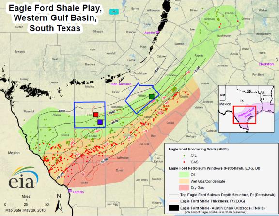
The productive Eagle Ford extends from the Mexican border (Webb to Maverick Counties) striking northeast to Brazos County, covering approximately 19,500 mi2. See Fig. 1. The Eagle Ford varies from approximately 14,000 ft deep and 300 ft thick in the southeast to approximately 4,000 ft deep and 50 ft thick as you move up dip to the northwest. Bottomhole temperatures range from 340ºF to 240ºF; hence, production is mainly gas in the deeper Eagle Ford, gas condensate, condensate, and oil as you move up dip. Mineralogy consists of mainly calcite, quartz, and illite, with minor amounts of pyrite, dolomite, plagioclase, mixed-layer clay, chlorite, and kaolinite. Detailed sedimentological and geochemical analyses of the Eagle Ford have documented substantial lithological and organic geochemical variability within the Eagle Ford that include total organic carbon (TOC), kerogen types, and mineralogy. Percentages of the major minerals vary greatly across the Eagle Ford and can vary drastically in the same county. Clay volumes vary from as low as 5% to as high as 35%, and calcite volume varies from 34% to 85%. In general, TOC ranges from 2.1 to 5.2 wt. %, Vitrinite Reflectance (Ro) ranges from an

2	SPE 159904

immature 0.68 to 1.5, core porosities vary from 1.5% to 9%, and log values average between 3% and 15%. Because of varying mineralogy, TOC, Ro, and porosity, it is essential to evaluate log data in conjunction with core data to establish models and determine if the Eagle Ford is economically viable.

Fig. 1—Eagle Ford Shale play map, courtesy of the U.S. Energy Information Administration.

In this paper, three Eagle Ford wells from Frio and Wilson Counties have been studied. The counties and wells are highlighted in Fig. 1. The shallowest well, Well 1, is indicated by the red square, the well at intermediate depth, Well 2, is marked by the green square, and the deepest well, Well 3, is shown by the blue square. The mineralogy (including TOC) for these wells is summarized in Fig. 2. By weight percent, there is an average of 57% calcite, approximately18% clay, with illite being the dominant clay, 15% quartz-feldspar, about 5% pyrite, and 4% TOC. The average fluid volumes (including kerogen) for these wells, determined from core analysis, are summarized in Fig. 3. In this case, kerogen volume was determined by correcting the TOC from Rock Eval Pyrolysis for the amount of free hydrocarbons in each core sample by using the Rock Eval S1. The average water-filled porosity is 2.25 pu, hydrocarbon fluid volume is 4 pu, and kerogen volume is 8 pu. The presence of such large amounts of kerogen complicates the interpretation by causing the grain density to vary. Underestimating kerogen results in the interpretation predicting too much hydrocarbon and, conversely, overestimating kerogen results in predicting too little hydrocarbon. It will be shown in a later section how NMR porosity can be used to confirm and improve the prediction of the kerogen volume.

SPE 159904	3

Fig. 2—Eagle Ford mineralogy for the three wells in this study.

Fig. 3—Eagle Ford average fluid volumes for the three wells in this study.

Fig. 4a—Eagle Ford core-grain density vs. core TOC.

Fig. 4b—Eagle Ford core porosity vs. core TOC.

4	SPE 159904

Figs. 4a and 4b show the relationship between core grain density, porosity, and TOC for the three wells. The red dots represent Well 1, the green dots represent Well 2, and the blue dots represent Well 3. The high amounts of TOC in the shallowest well are consistent with the source rock in this well having the lowest value of Ro. Each well displays a weak trend of grain density decreasing with TOC, but the trends for each well are different. Note the variation in grain density when the weight percent TOC is less than 5. If an interpretation is made with the assumption of constant grain density, a porosity error of 5 pu will result. However, in a later section, it will be shown how a good estimate of grain density can be obtained using geochemical well log data. The weak correlation of porosity with TOC for all the wells suggests that much of the porosity is matrix porosity, not porosity associated with the organic matter.

Dielectric Logging and Interpretation

The dielectric measurements in this paper were obtained with a new formation-evaluation sensor that operates in the microwave range (1 GHz) to differentiate reservoir fluids (Bittar et al. 2010). The sensor consists of three receiving antennas located between two transmitting antennas. All five antennas and related electronics are mounted in an articulated pad that is extended toward the formation. The electronic and signal processing provide logs of formation dielectric constant and formation conductivity, which can be used to calculate the bulk volume of water in the flushed zone. The configuration of the antennas compensates for tool standoff, mud cake effects, and borehole rugosity.

An electromagnetic wave propagating through a material will be attenuated and experience a phase shift. Both of these can be measured (Bittar et al. 2010) and converted by means of a table to look up the formation resistivity, R, and dielectric constant of the material, ε’. The imaginary dielectric constant, ε’’, can be derived from the formation resistivity, R. Table 1 provides the real and imaginary dielectric constants for several materials encountered in formation evaluation. The upper bound for the real dielectric constant for kerogen, 3.3, is from Seleznev et al. (2011), and the values for clay, 5–6, are from Schmitt et al. (2011). The high value of the real dielectric constant of water makes the measurements particularly sensitive to water filling the porous space; consequently, one of the natural applications of dielectric logging is the measurement of water-filled porosity in the near-wellbore region, with little or no dependence on the water salinity and Archie electric parameters, m and n (Schmitt et al. 2011).

TABLE 1. DIELECTRIC CONSTANT FOR SEVERAL MATERIALS ENCOUNTERED IN

FORMATION EVALUATION.

Material	Real Dielectric Constant ε’	Imag. Dielectric Constant ε’’ (1Ghz)
Water	56–80	0.2–20
Air, Gas	1	0.0
Oil	2.0–2.2	0.0
Kerogen	2.2–3.3	0.0
Sandstone	4.65	0.1
Limestone	7.5–8	0.01
Dolostone	6.8	0.01
Anhydrite	6.3	0.001
Pyrite	80	200
Clay	5–6	.1–.25

The most widely used approach for interpreting dielectric data is the complex refractive index method (CRIM) model. The key equations are clearly documented in Bittar et al. (2010) or Schmitt et al. (2011). In our interpretations, the key CRIM parameters are the matrix real and imaginary dielectric constants, the assumed salinity of the water in the zone investigated by the tool, and the total porosity. The matrix real and imaginary dielectric constants can be obtained from the mineralogy by solving for mineral volumes from geochemical elemental logs (Galford et al. 2009) using Table 1 and applying Eq. 3 (next section) from Bittar et al. (2010). The salinity can be obtained from samples or by interpretation so that the dielectric and total porosities overlay in zones devoid of hydrocarbon. Alternatively, the salinity can be obtained from inversion of the CRIM equations and then making a second interpretation with the salinity constrained around this value (Schmitt et al. 2011). The following CRIM equation is used to compute the flushed-zone water saturation, from which, in conjunction with the

porosity, the flushed-zone water-filled porosity (water-filled dielectric porosity), φSxo , can be computed as:

Sxo =	ε*for	−(1−φ)	εmatrix*	−φ εHC*
		φ( εmf*	− εHC* )
				(1)
φDielectric =φS		xo
water

SPE 159904	5

Where, ε*for is the measured complex dielectric constant obtained by measuring the phase and attenuation of the EM wave;

εmatrix* ,εHC* are the matrix and hydrocarbon complex dielectric constants; εmf* is the complex dielectric constant of mud filtrate in the zone investigated by the tool (a function of temperature and salinity); φ is the formation total porosity, and Sxo

is the water saturation of the flushed zone. For completeness, the apparent water-filled dielectric porosity can be defined (Bittar et al. 2010) as:

		ε*	−	ε*
	φwaterCRIM =	for		matrix	(2)
		ε*	−	ε*
		mf		matrix

The apparent water-filled porosity,φwaterCRIM , can be computed solely from the dielectric sensor measurements and should

overlay total porosity, φ, in zones devoid of hydrocarbon or TOC. However, the apparent water-filled dielectric porosity, φwaterCRIM , is not the same as the dielectric water-filled porosity,φwaterDielectric , obtained from the CRIM in Eq. 1.

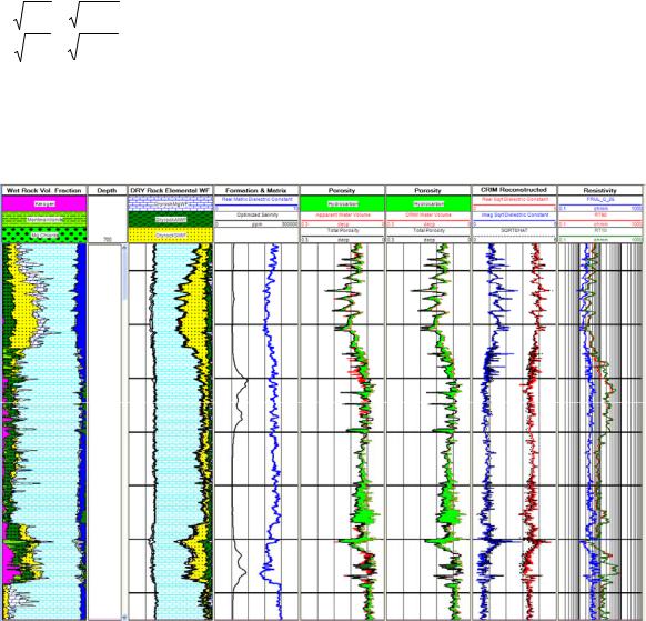
Fig. 5—CRIM method applied for interpretation of dielectric well log data.

Fig. 5 summarizes the results of applying the CRIM method for computing the water-filled dielectric porosity for Well 1. Track 1 presents the mineralogy obtained from the geochemical well log data, and Track 2 presents the raw elemental weight fractions. The three primary elements are calcium (light blue), silicon (yellow), and aluminum (green). The blue curve in Track 3 is the real part of the matrix dielectric constant, computed from the mineralogy and can be seen to vary as the carbonate fraction varies. The red curves in Tracks 4 and 5 are the apparent water-filled dielectric porosity and the waterfilled dielectric porosity, respectively. Total porosity is from the interpretation in Track 1, and the shading represents the CRIM volume of hydrocarbon, which, for the most part, agrees with the hydrocarbon volume in Track 1. In addition to obtaining the water-filled dielectric porosity, the salinity is determined and shown in Track 3. Track 6 displays the square root of the real (red) and imaginary (blue) components of the formation dielectric constant. The dotted black lines represent the predicted square root of the real (red) and imaginary (blue) components of the formation dielectric constant using the CRIM equation. Track 7 presents the deep and shallow resistivities along with the dielectric resistivity (blue). The dielectric resistivity is always less than the deep induction resistivity owing to spreading loss, not as a result of mud-filtrate invasion, which is minimal in these wells.

φwaterDielectric

6	SPE 159904

Geochemical Logging and Interpretation

The geochemical measurements used in this paper were obtained with a new logging tool (Galford et al. 2009a; Galford et al. 2009b). The tool provides measurements of elemental weight fractions of the elements magnesium, aluminum, silicon, potassium, calcium, titanium, manganese, iron, and gadolinium important to mineralogical analysis of rock formations and geochemical stratigraphy.

The mineralogical interpretation involves “turning the measured elemental weight fractions into minerals.” By using the aluminum and magnesium elemental weight percentages not previously measured from spectroscopy logging, there is greater assurance that the lithology is correctly identified, and the interpretation is enhanced by providing volumetric estimates of the specific types of clay and other minerals in the formation. The resulting mineral volumetric fractions (including kerogen) can be used to compute, at each depth, the square root of an apparent complex matrix dielectric constant:

ε*	=	∑Vi εi*
		i			(3)
			∑Vi
matrix
			i
Where, Vi are the volumes of each of the minerals (including kerogen) in the mixture, and					εi* are their corresponding
complex dielectric constants. The square root of the complex matrix dielectric constant, εmatrix*					, can then be used in Eqs. 1

and 2 to solve for the flushed-zone water saturation, Sxo, the dielectric water-filled porosity,φwaterDielectric , and the apparent water-

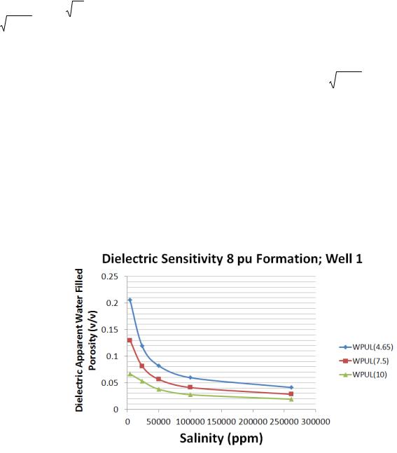
filled porosity, φwaterCRIM , respectively as discussed in the previous section and shown by Fig. 5. Fig. 6 shows the significance of using the correct matrix dielectric constant when solving for the dielectric water-filled porosity. The y-axis presents the

dielectric apparent water-filled porosity, , and the x-axis presents formation water salinity in ppm. The data are

computed for Well 1 at a depth where the total porosity is approximately 8 pu. The blue, red, and green curves correspond to a matrix dielectric constant of 4.65, 7.5 and 10, respectively. The real matrix dielectric constant, plotted in Track 3 of Fig. 5, varies from about 5.5 to 8 for this well. Assuming a salinity of about 75,000 ppm, Fig. 6 shows that as the matrix dielectric constant varies from 5.5 to 8, the dielectric apparent water-filled porosity varies from about .055 v/v to .035 v/v, or about a 2 pu variation. Using a matrix dielectric constant of 5.5 when the actual is 8 would result in overestimating the water-filled porosity and underestimating the hydrocarbon volume by 2 pu. Using the mineralogy determined from the geochemical log to estimate the matrix dielectric constant will help avoid such errors.

Fig. 6—Sensitivity of CRIM dielectric apparent water-filled porosity to salinity and matrix dielectric constant.

SPE 159904	7

Fig. 7—Well 3 interpretation based on geochemical, neutron, density, and resistivity logs.

Fig. 7 presents the results of an interpretation based on geochemical, neutron, density, and resistivity logs for Well 3. Track 1 presents the raw elemental weight fractions, and Track 2 presents the mineralogy. The three primary elements in Track 1 are calcium (light blue), silicon (yellow), and aluminum (green). Track 3 compares the predicted porosity with core data. Predicted porosity can seem to be as large as 13 pu. Track 4 compares the predicted grain density with core-grain density. The grid lines represent 100-ft intervals, and core data shows the grain density can vary from a low of 2.38 g/cc to a high of 2.73 within this 100-ft interval owing to variations in the mineralogy and TOC. Track 5 compares TOC with core data, and Track 6 compares the interpreted water saturation to core data. The interpreted fluid volumes are presented in Track 7, where each vertical division represents 6 pu. The magenta shading represents the kerogen volume, grey shading represents clay-bound water, blue shading represents water, and green shading represents oil. The yellow curve is the NMR total porosity. The NMR porosity generally agrees very well with the interpreted total porosity (all the shaded areas in Track 7 excluding the magenta) and is an independent confirmation of the interpreted porosity (Track 3).

Before leaving this section, we note that, while the mineralogy is of interest, the primary use of obtaining an accurate mineralogy is to compute an accurate grain density. Grain density can by predicted from the mineralogy using the following equation:

	1		Wker ogen			n	W
		=				+∑		min−i	(4)
ρ				ρ			ρ
	grain _ density				ker ogen	i=1		min−i

Where, Wmin-i are the bulk dry rock mineral fractions, and Wkerogen is the bulk dry-rock mineral fraction of kerogen. The mineral densities, ρmin-i, are parameters to be determined, but are known for many of the minerals, such as calcite and quartz. When accurate XRD or XRF data is available, the mineral densities can be estimated using the following equation:

	m	1		Wker ogen, j		n	Wmin−i, j	2
			−		−	∑i =1			(5)
		ρgrain _ density, j		ρker ogen			ρmin−i
	∑j =1

Where, subscript, j, is a counter for the number of core samples, Wmin-i,j are the XRD bulk dry-rock mineral fractions, and Wkerogen,j is the bulk dry-rock mineral fraction kerogen for the jth core sample, and ρgrain_density,j is the core grain density for the

8	SPE 159904

jth sample. The unknown mineral densities ρmin-i are the unknowns in Eq. 5 and can readily be obtained using a constrained optimization approach, such as is available in the Excel Solver. The constrained optimization approach allows one to fix the expected densities for some known minerals, such as quartz and pyrite, and focus on the more variable clay mineral clay densities.

NMR Interpretation for Porosity, Kerogen Volume, and Hydrocarbon Volume

NMR logging, when combined with neutron, density, and dielectric logs, provides an independent method of determining kerogen and hydrocarbon volume in shale reservoirs. Both the neutron and density porosities are approximately the sum of

the formation water, hydrocarbon, and kerogen volumes; consequently, both the density porosity,φDensity , or crossplot

porosity, φxplot , are too large by an amount approximately equal to the kerogen volume. NMR logging tools are sensitive to

protons, but only to those in rapid motion (Herron et al. 2011). The hydrogen protons contained in the formation matrix and kerogen are invisible or undetected by the NMR logging tool (Ramirez et al. 2011). Thus, NMR logging tools are sensitive to pore fluids, but insensitive to hydrogen protons in minerals and kerogen and the NMR total apparent formation porosity is independent of mineralogy.

In general, NMR porosity may be affected by hydrogen index and insufficient polarization time, both of which would potentially cause NMR porosity to read too low. In organic-rich source rock reservoirs, both of these effects have been shown to be minimal, and it is expected that NMR porosity will provide a close match to core porosity, even in gas-shale reservoirs. This is consistent with observations in the Haynesville Shale (Ramirez et al. 2011) and with lab measurements in the Barnett Shale (Sigal and Odusina 2011). For the three oil-window Eagle Ford wells studied in this paper, there is good agreement between the NMR log porosity and core porosity, as shown in Fig. 8. Fig. 8 shows the comparison between core porosity (red points) and NMR total porosity, T2PTOT, (black curve) for all three wells; Well 1 is shown in Track 2, Well 2 is shown in Track 5, and Well 3 is shown in Track 8. Based on these observations, it is possible to use the NMR porosity as a minimum porosity constraint in the integrated petrophysical analysis. Track 7 of Fig. 6 shows that the NMR porosity generally agrees very well with the interpreted total porosity, as previously discussed in the Geochemical Logging and Interpretation section.

Fig. 8—Comparison of NMR log data to core porosity for all three wells. From left to right, Well 1, Well 2, and Well 3.

Because both the neutron and density porosities are affected by the presence of kerogen, but kerogen is undetected by NMR logs, it follows that an estimate of the kerogen volume can be obtained from the density, neutron, and NMR tools using

Eq. 6. An approach similar to Eq. 6 for obtaining Vkerogen was proposed by Herron et al. (2011) and uses the density porosity rather than crossplot porosity. Fig. 8 also shows the comparison between core kerogen volume (red points) and Vkerogen

estimated from Eq. 6 with a “c” of 1 (blue curve) and Vkerogen estimated from the difference between density porosity and

NMR porosity with a grain density of 2.71 g/cc and a “c” of 1 (black curve); Well 1 is shown in track 3, Well 2 is shown in track 6, and Well 3 is shown in track 9.

Vker ogen ≈cφxplot −φNMR

(6)

SPE 159904	9

Because NMR porosity is a close match to core porosity, it provides a good estimate of total reservoir fluid volume, including water and hydrocarbon. The dielectric log provides an independent measure of water-filled porosity. The NMR and

dielectric measurements can be combined, as shown in Eq. 7, to estimate Vhydrocarbon , the hydrocarbon-filled porosity. Adding Eqs. 6 and 7 together provides Eq. 8:

V		≈φ	NMR		−φCRIM			(7)
hydrocarbo n						water
V	+V			≈cφ		xplot	−φCRIM ≈V	(8)
kerogen	hydrocarbons						water TOC

In Eqs. 2 and 3, the square root of the complex matrix dielectric constant, εmatrix* , can be assumed to be constant or

adjusted for the volume of kerogen. The “c” in Eqs. 6 and 8 is a normalizing constant, adjusted so that cross-plot and NMR porosities overlay in zones devoid of hydrocarbon. The proposed quick look can be compromised by any of the uncertainties

affecting φxplot (matrix density, hydrocarbon density, crossplot porosity computation), φNMR (hydrogen index, “invisible”

clay-bound water), and φwaterCRIM (matrix complex dielectric constant, assumed salinity, CRIM equation), but should nevertheless prove useful for a quick reconnaissance interpretation. Finally, it follows that in general:

φwaterDielectric ≤φNMR ≤φ

(9)

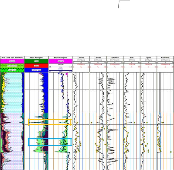
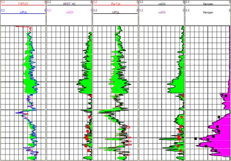
Fig. 9—Well 2 interpretation based on geochemical, neutron, density, and resistivity logs.

Fig. 9 presents the results of an interpretation based on geochemical, neutron, density, and resistivity logs for Well 2. TOC can be obtained using the Delta LogR approach of Passey (1990), or from regression to bulk density or uranium from well log data. The geochemical logs and TOC are used for obtaining the mineralogy weight fractions from which the grain density can be obtained. Fluid volumes, referred to as “the interpretation,” are obtained from the neutron, density, and resistivity logs. Track 1 presents the mineralogy obtained from the geochemical well log data. The interpreted fluid volumes are presented in Track 2, where each vertical division represents 6 pu. The magenta shading represents the kerogen volume, grey shading represents clay-bound water, blue shading represents water, and green shading represents oil. The yellow curve is the NMR total porosity. Track 3 compares the Track 2 kerogen with two other predictors of kerogen: 1) the blue curve predicts kerogen from the difference between cross-plot porosity and NMR porosity, Eq. 6, using a “c” of 1.0; 2) the black curve predicts kerogen from the difference between density porosity and NMR porosity using a grain density of 2.71 and a “c” of 1.0. The scale in Track 3, from left to right, is from 0.2 to -0.05 v/v. This is done to demonstrate that the models are properly calibrated. Tracks 4 through 9 compare the mineral dry weight-percent fractions for quartz, calcite, dolomite, illite,

10	SPE 159904

pyrite, and kaolinite with core XRD data. Focusing on the area within the blue rectangle, it can be seen in Track 2 that the NMR porosity is approximately 3–4 pu larger than the interpreted porosity, and in Track 3, the kerogen from NMR-cross-plot porosity and NMR-density porosity is about 3–4 pu smaller than the interpreted kerogen. Mineralogy is fairly constant throughout this interval of the well, so it is possible that the interpreted kerogen is too high and the interpreted porosity is too low. The validity of this statement is confirmed by the core porosity (not shown). Focusing on the area within the orange rectangle, the interpreted porosity, Track 2, is seen to be significantly greater than the NMR porosity (yellow curve) and most likely too large for so much clay. Again, some of this could be a result of underestimating the valid amount of kerogen.

Fig. 10 compares the NMR-dielectric oil volume with the interpreted oil volume obtained from the standard-response equation inverse technique using the geochemical, porosity, and resistivity logs for Well 1. Track 1 presents the NMR total

porosity and the apparent water-filled porosity, φwaterCRIM (blue curve), with green shading indicating hydrocarbon volume. Track 2 presents the Track 1 hydrocarbon volume and compares it with core data (red dots). Track 3 presents the interpreted geochemical, nuclear log porosity, φ, and the apparent water-filled porosity, φwaterCRIM (blue curve), with green shading

indicating hydrocarbon volume. Track 4 presents the interpreted hydrocarbon volume from the standard response equation inverse technique using the geochemical, porosity, and resistivity logs, and compares it with core data (red dots). In this particular case, the NMR-dielectric hydrocarbon volume, Track 2, agrees better with the core data. Track 5 presents the interpreted kerogen volume and compares it with core data.

Fig. 10—Comparison for Well 1 of hydrocarbon volume from NMR-dielectric (Track 2) with hydrocarbon volume from geochemical, porosity, and resistivity logs (Track 4).

Looking at all Three Interpretations

In this section, we summarize and compare the interpretations for all three wells. Recall, the shallowest well is Well 1, the well at intermediate depth is Well 2, and the deepest well is Well 3. All three wells have complete logging runs, including geochemical, NMR, neutron, density, and resistivity data. Only Well 1 has dielectric data. The previous sections suggest using an interpretation workflow, as defined in Fig. 11. The workflow shown in Fig. 11 suggests using, initially, two almost independent approaches: one using geochemical, nuclear, acoustic, and resistivity logs and a second using NMR and dielectric logs and in addition cross-plot porosity and NMR to determine kerogen volume. After the parameters are adjusted for consistency between the two approaches, all the measurements can be combined into a single interpretation using constraints and statistical optimization techniques. However, this was not done in obtaining the results shown in Fig. 12.