Прямой доступ к библиотеки Приложений.

Чтобы получить прямой доступ к библиотеки Приложений необходимо:

1. Из Меню Файлов кликнуть Открыть (Open).

2. В ящике Диалогов. Кликнуть кнопкуFavorites.

3. Кликнуть appdirectory.

4. Просмотреть описание файла, кликнуть файл, а затем кликнуть Previewbuttonв открытом ящике линейки инструментов (boxtoolbar).

5. Кликнуть файл, который вы хотите открыть. Затее кликнуть Open.

6. Загружаются вход и результаты. Вы можете проверить, модифицировать и запустить моделирование.

Проверка Описания файлов.

Чтобы просмотреть описание файла перед его открытием необходимо:

1. Изменю Данные (Data), кликнутьSetup, а затем кликнутьSpecifications.

2. Кликнуть лист Описаний (Descriptionshee)

Чтобы проверить доступные комментарии для блоков и других объектов, кликнуть кнопку Комментарии (Commentsbutton) из линейки инструментов Обозревателя данных

(DataBrowser).

Если комментарии доступны, кнопка комментарии (Commentsbutton) выглядит следующим образом:.

Если комментарии не доступны , кнопка выглядит следующим образом:

Создание ориентированных на проблем уравнений (Creating an Equation Oriented

Problem).

Метод ориентированных уравнений (ЕО) доступен для решения опций Аспен плюс.

Как всегда, Технологическая схема конфигурируется с помощью Графического Интерфейса Пользователя (GUI). Связность Технологической схемы определяется при графическом построении технологической схемы и Проводник данных используется для конфигурирования блоков и потоков.

ЕО требует дополнительного входа через Проводник данных (DataBrowser).

Перед решением вашей схеме в ЕО, однако, вы должны инициировать ее в SM.

Это не требует полного решения в SM, однако, минимальное требование в том, что каждый блок решается однажды. Это обеспечивается начальными условиями для ЕО переменных. Как тесноSMтехнологической схемы нуждается в решении зависти от строгости формулировки ЕО проблемы.

Создание и исследование модели технологической схемы совместно с системами автоматического управления на примере схемы получения метилциклогексана.

Для решения этой задачи необходимо создать схему получения метилциклогексана в программном комплексе Аспен Плюс, промоделировать схему в стационарном режиме, а затем выполнить моделирование схемы в динамическом режиме. При моделировании схемы в динамическом режиме необходимо дополнить модель схемы необходимыми данными для моделирования процесса в динамическом режиме, а именно, размерами тарелок, габаритами конденсатора. кипятильника и сборников, для того, чтобы иметь возможность наблюдать поведение отдельных аппаратов и схемы в целом при действии различных возмущений.

Для создания задачи моделирования стационарного режима работы необходимо выполнить следующие действия

1.Открываем AspenPlus,появляется диалоговое окно:

ставим флажок Template.

2. В меню Simulations выбираем General with English Unit, в меню Run Type выбираем Flowsheet.

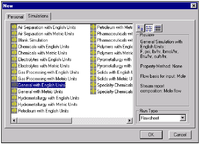
3. Нажимаем OK.

4. В поле рисунка (ProcessFlowsheetWindow) создаем схему.

5. В меню библиотек (ModelLibrary) выбираем вкладкуColumnsдалееRadFrac

6. Нажимаем стрелку справа от столбца RadFrac, появляется окно модификаций.

7. Выбираем FRACT1 и перетаскиваем его (нажмите и удерживайте) в поле технологической схемы (создается блок В1).

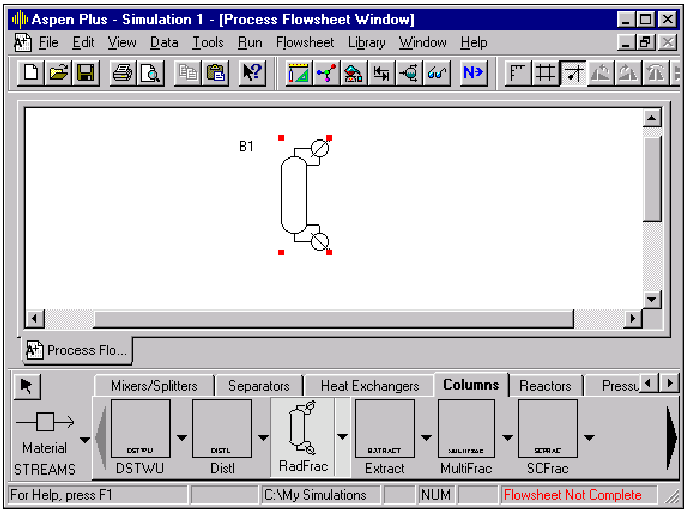
8. Далее перейдем в меню потоков и выберем материальные потоки (MaterialStreams):

9. Появляются порты (стрелки) на блоке В1, которые совместимы с потоком.

10. Подводим курсор к нужной стрелке и нажимаем на нее, далее нажимаем в свободной области технологической схемы, появляется поток 1.

11. Создаем другой материальный поток (поток 2) соединяющийся с блоком B1 в том же самом порту, что и поток 1, повторяя п 8-10.

12. Аналогично создаем потоки 3 и 4

Добавление Данных к Модели Процесса

1. Нажимаем кнопку «далее». Появляется диалоговое окно Flowsheet Complete

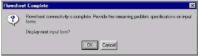
2. Нажимаем OK, чтобы показать первую необходимую вкладку.

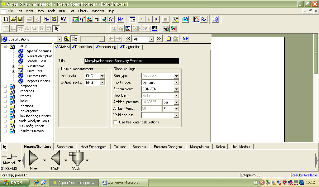
Setup\Specifications\Global:

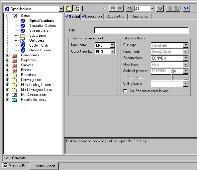
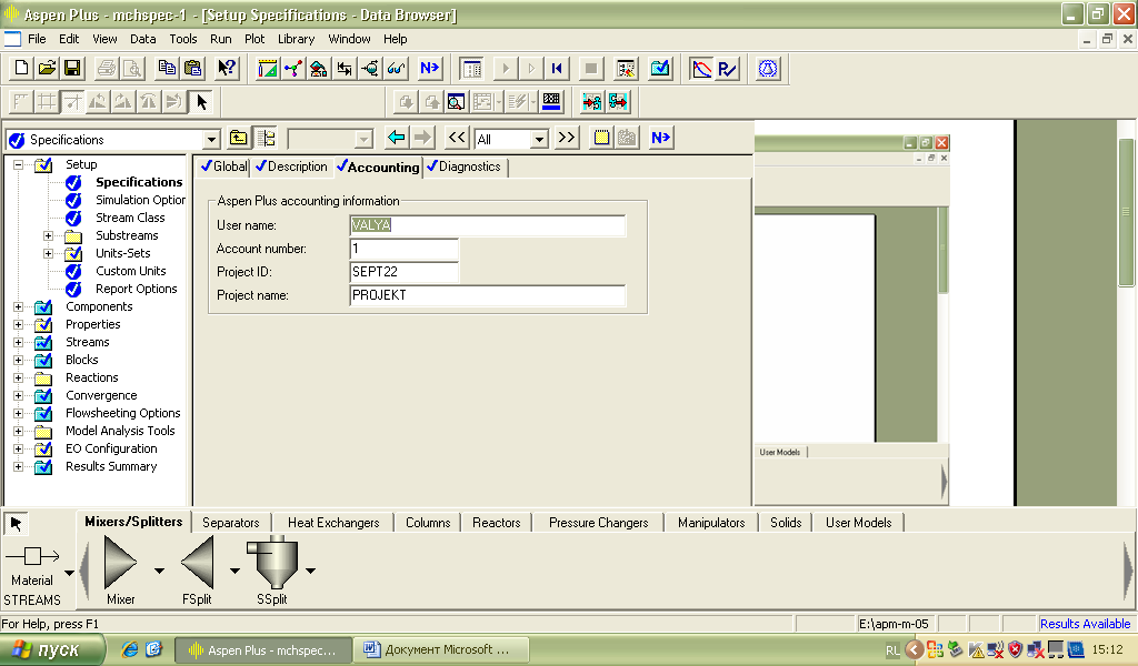
А также заполняем вкладку Accounting(информация о создателе проекта)

3. В поле Title, вводим текстMethylcyclohexane Recoveryи нажимаемEnter

4. Перемещаемся далее Setup \Report Options \ General, щелкая по соответствующей вкладке, мы можем настраивать создание отчетов для определенных частей моделирования.

5. Нажимаем на вкладку Stream.

6. Устанавливаем флажки как показано на рисунке:

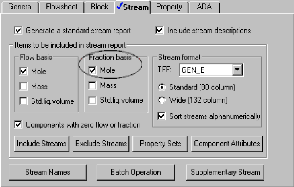
Теперь Aspen Plus будет рассчитать и представить мольные доли всех компонентов потоков.

7. Нажимаем на кнопку Property Sets.

8. Выбираем TXPORT и перемещаем стрелочкой в Selected property sets

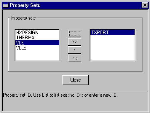
9. Нажимаем Close.

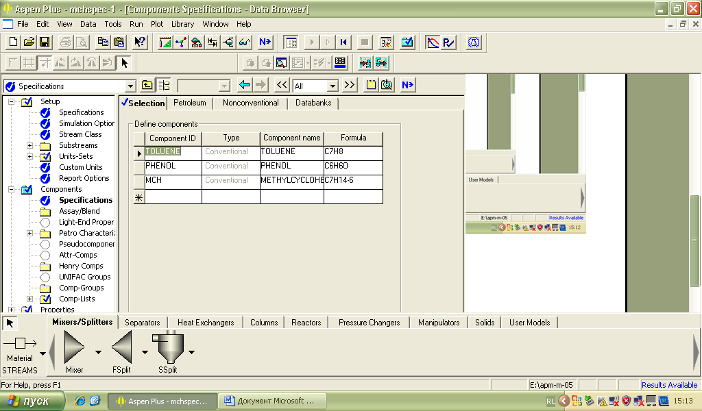
10. Нажимаем кнопку «далее» и переходим Components \ Specifications \ Selection, производится ввод компонентов.

1. В поле Component ID вводим TOLUENE, и нажимаем Enter(остальные поля заполняются автоматически).

2. В следующем поле Component IDвводим PHENOL , и нажимаем Enter(остальные поля заполняются автоматически).

3. В следующем поле Component ID, вводимMCHи нажимаем Enter(т.к.Aspen Plus не распознает сокращение MCH поэтому остальные поля не заполнены).

4. В строке компонент MCH, вводим METHYLCYC и нажимаем Enter. Появляется диалоговое окно со списком всех компонентов в Aspen Plus данных, которые имеют имя, содержащее METHYLCYC:

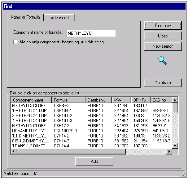
5. В списке, находим и выбираем Methylcyclohexane.

6. Нажимаем кнопку Add.

7. Нажимаем кнопку close.

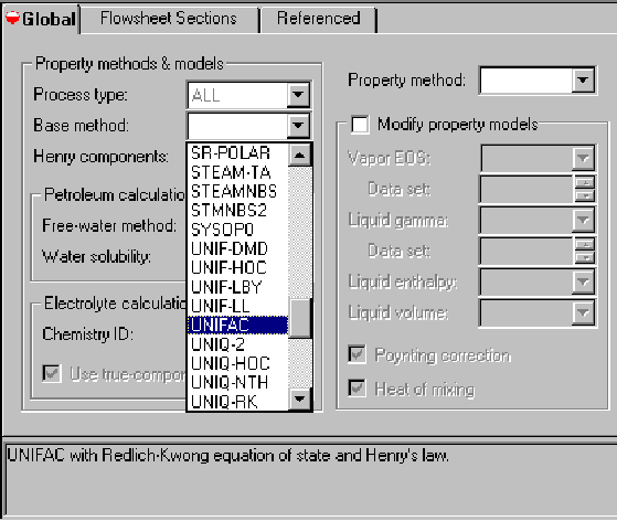
8. Нажимаем кнопку «далее» и переходим Properties \ Specifications \ Global

Выбор термодинамических методов

1. В списке Base method, используя вертикальную полосу прокрутки и, выбираем UNIFAC.

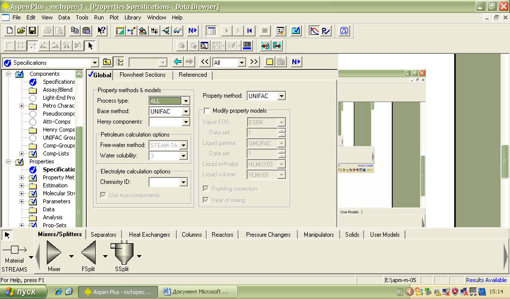
2. Нажимаем кнопку «далее», появляется диалоговое окно Required Properties Input Complete

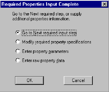
3. Нажимаем OK.

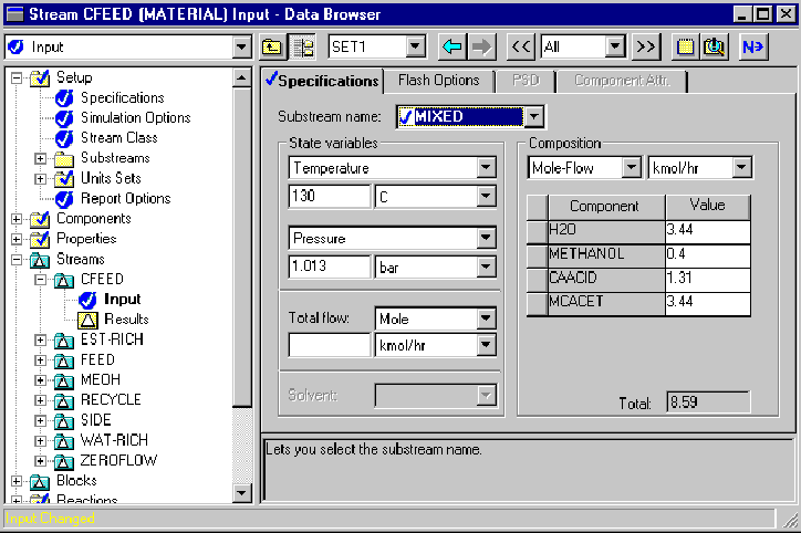
Переходим в меню Streams \ 1 \ Input \ Specifications

1. Вводим следующие переменные состояния для потокаMCH-Toluene:

температура 220 F

давление 20 psi

Toluene200lbmol/hr

MCH 200 lbmol/hr

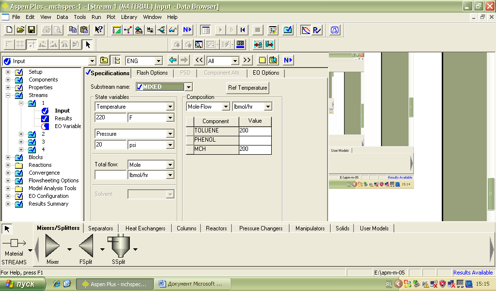
2. Нажимаем кнопку «далее».

Streams \ 2 \ Input \ Specifications Вводим следующие параметры:

температура 220 F

давление 20 psi

Phenol1515,08lbmol/hr

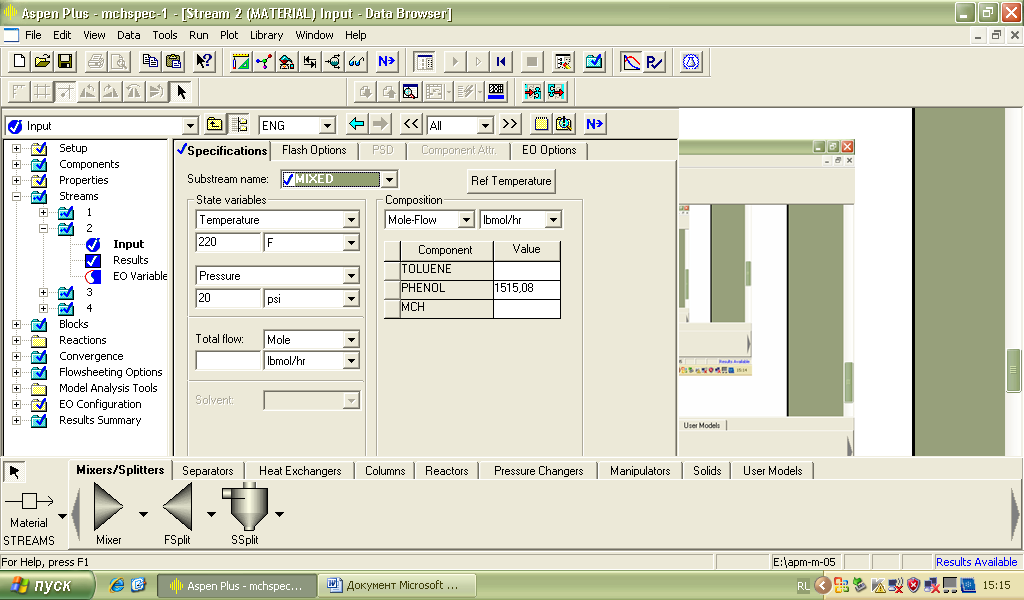
3. Нажимаем кнопку «далее».

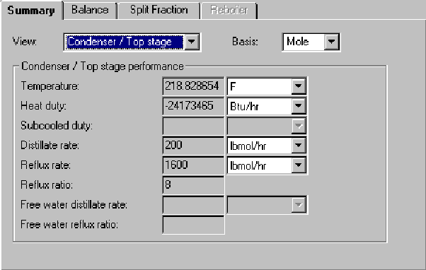
Blocks \ B1 \ Setup \ Configuration :

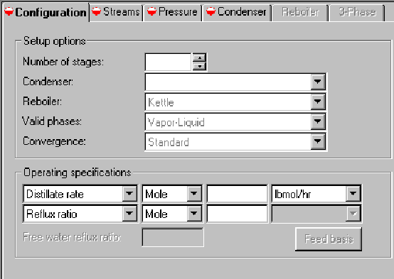
4. Enter the following specifications for the column:

В поле Number of stages устанавливаем значение22

В поле Condenserустанавливаем Total

В поле Distillate rate устанавливаем значение200 lbmol/hr

В поле Reflux ratioустанавливаем значение 8

5. Нажимаем кнопку «далее» или переходим на вкладку потоков.

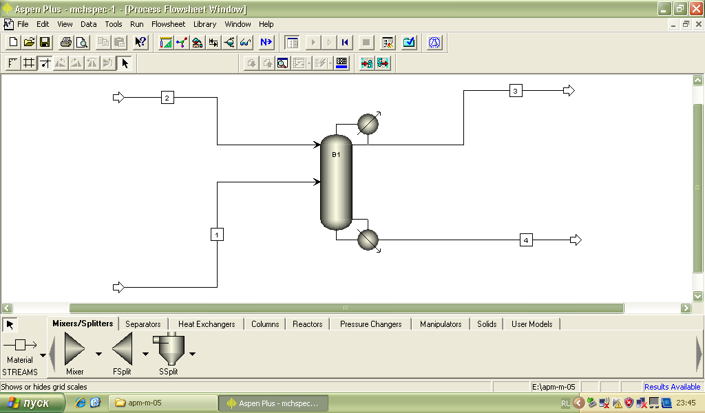
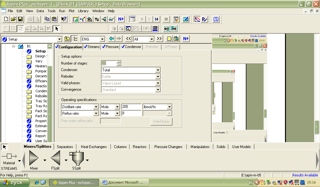
Blocks \ B1 \ Setup \ Streams В модели RadFrac, есть N тарелок. Тарелка 1 является верхней стадией(Конденсатор); тарелка N является нижней ступеней (испаритель). Какпоказано на рисунке 3.1, MCH-толуол - тарелка 14, и фенол - тарелка 7.

6. Вводим 14 в поле stageдля потока 1.

7. Вводим 7 в поле stageдля потока 2.

8. Нажимаем кнопку «далее».

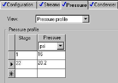
Blocks \ B1 \ Setup \ Pressure

8. В поле View выбираем Pressure profile.

9. В поле Stage вводим 1, затем нажимаемTab.

10. В поле Pressureвводим значение 16 и затем нажимаемTab.

11. Далее в Stage вводим 22, затем нажимаемTab.

12. В поле Pressureвводим значение 20.2

8. Нажимаем кнопку «далее».

Запуск симуляции

1. В появившемся диалоговом окне Required Input CompleteнажимаемOK.Панели управления и запуск моделирования начинается:

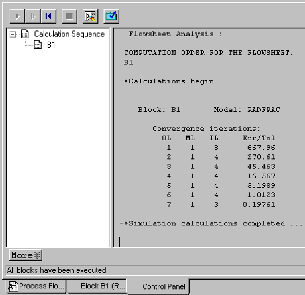
Проверка результатов моделирования

1. Перейдем в окно технологической схемы.

2. В технологической схеме, выбираем блок В1, щелкаем правой кнопкой мыши для отображения контекстного меню.

3. В контекстном меню выбираем Results.

Block B1 Results Summary:

Результаты представлены по трем формам: Results Summary, Profiles, и Stream Results .

4. Выбираем Blocks \ B1 \ Profiles щелкнув один раз на любой профиль или его галочкой, появляется лист Block B1 Profiles TPFQ - отчетность по температуре, давлению, теплу:

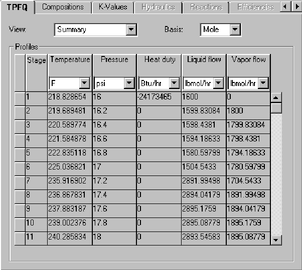
5. Здесь можно просмотреть результаты, поменять единицы измерения.

Динамика

Если на панели инструментов нет кнопки DynamicToolbarкак показано на рисунке:

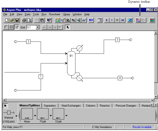то выполните следующие шаги, чтобы добавить панель инструментов: убедитесь, что окно схемы активно, заходим в меню View → Toolbarв диалоговом окне выбираемDynamic:

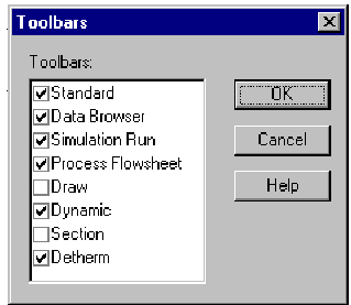
Нажимаем кнопку ОК. Динамическая панель инструментов добавляется к панели инструментов.

-Нажимаем , после этого мы получаем доступ к вводу динамических данных. Нажимаем кнопку "Далее" и появляется диалоговое окно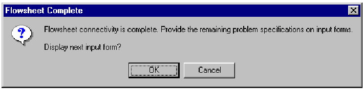

- Нажимаем, кнопку ОК Браузер данных начинается с блока B1 (RADFRAC) вкладка Reflux Drum

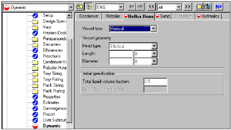
1. В поле Vesseltype, выберите из спискаHorizontal.

2. В полеLengthустанавливаем значение 6 футов и в полеDiameter- 3 фута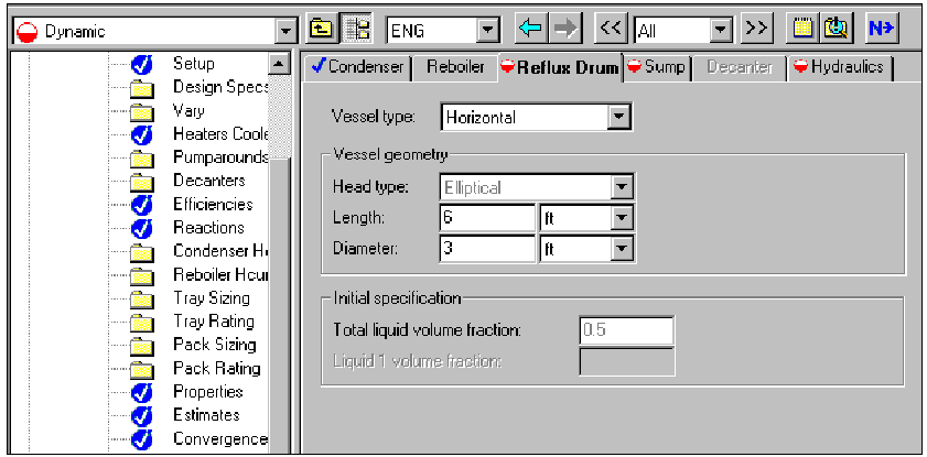

3. Нажимаем кнопку далее.

4. Переходим на вкладку Condenser

5. В окне вариант передачи тепла, в ниспадающем окне выбираемиз спискаLMTD.

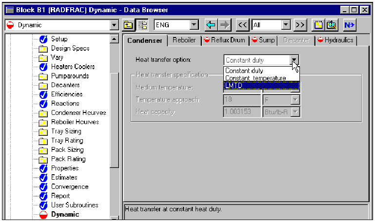
6. Нажимаем далее, переходим на следующую вкладку грязевик листа появляется.

7. В поле Lengthустанавливаем значение 5 футов и в полеDiameter- 3 фута. Не изменяйте другие значения.

8. Нажимаем клавишу Enter, чтобы принять ввод.

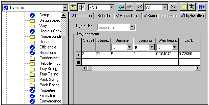
9. Нажимаем Далее, чтобы перейти на вкладку Hydraulics

10. В Stage1 установим значение 2, в Stage2 - 21.

11. В столбце Diameter, удалить 6,56168 и установить значение 5.

12. Нажимаем клавишу Enter, чтобы принять вход, оставив остальные значения по умолчанию.

13. Нажимаемдалее, чтобы продолжить. Появляется диалоговое окно:

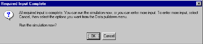
14. Нажимаем кнопку ОК. Aspen Plus отображает панель управления, где вы можете просмотреть сообщения омоделировании во время запуска.

15. Подождите, пока моделирование завершиться.

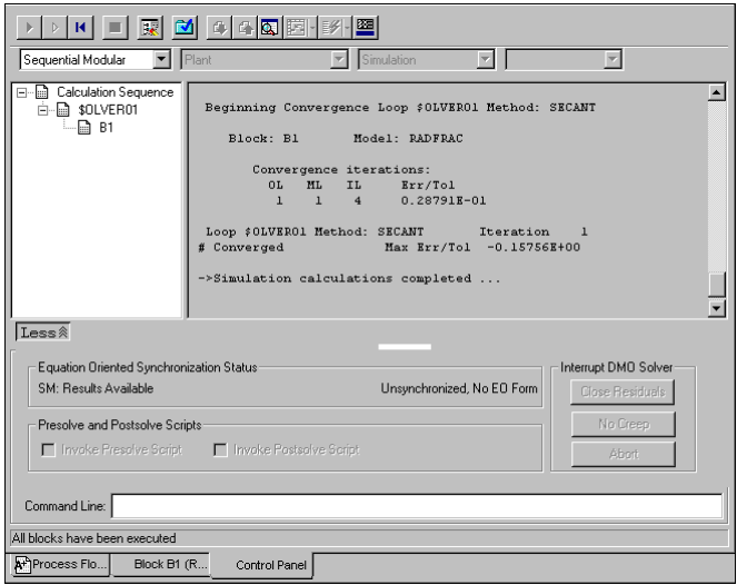
16. Нажмите кнопку «Закрыть», чтобы закрыть окно «Панель управления».

Сохранение и экспорт файла:

1. В меню File выбираем команду Export

2. Выбираем формат файлов (*. dynf).

3. В поле «Имя файла» вводимmchspec-1

4. В меню File выберите команду «Сохранить как».

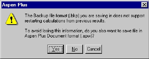
5. В поле «Сохранить как», выберите формат файлов (*. BKP).

6. В поле «Имя файла» введитеmchspec-1 нажмите кнопку «Сохранить». Появится диалоговое окно, запрашивающее, если вы хотите сохранить файл вAspen Plus документа (быстрый перезапуск) формате.

Открываем AspenDynamics

На следующем рисунке показана рабочая область AspenDynamicsсостоящая из трех окон:

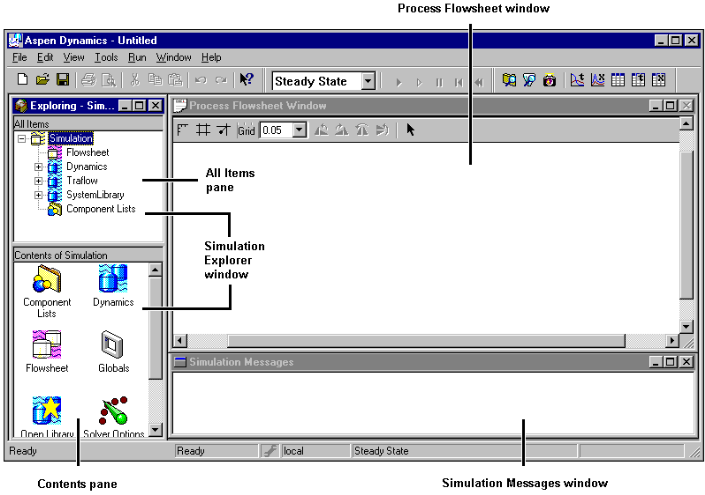
Окна Aspen Dynamics: • окно технологической схемы (Process Flowsheet Window) • окно сообщений моделирования (Simulation Messages Window) •окно Simulation Explorer Window, которое включает все элементы панели(библиотеки или папки модели) и содержание панели (все отдельные объекты выбранной библиотеки или папки).

Открытие файла mchspec-1.

1. Меню File → Open.

2. В появившемся диалоговом окне найдем файлmchspec-1, который мы экспортировали с расширением (*. dynd,*.dynf).

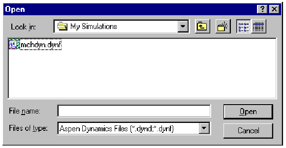
3. Выбираем mchspec-1, затем нажимаем кнопку «Открыть», чтобы загрузить mchspec-1.

Добавление нового контроллера

1. В библиотеке AllItemsнайдем библиотеку Dynamics.

2. Находим библиотеку ControlModels.

3. Из списка ControlModels, выбираем объект PID.

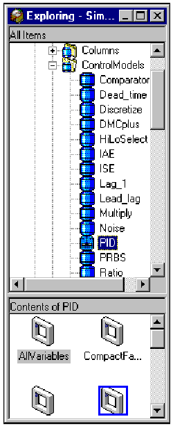
4. Перетащим PID на окно технологической схемы и поместим его над потоком 2 .

5. Нажмем на этот блок, чтобы выбрать его.

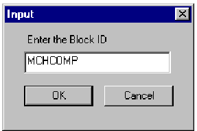
6. Щелкнем правой кнопкой мыши на блоке в появившемся меню выберем команду Rename.

7. В диалоговом окне ввода, вводим новое имя контроллера MCHCOMP, затем нажимаем кнопку ОК.

Добавление блока DeadTime:

1. В библиотеке Control Models выбираем объект Dead_time и перетаскиваем его на технологическую схему.

2. Нажмем на этот блок, чтобы выбрать его.

3. Щелкнем правой кнопкой мыши на блоке в появившемся меню выберем команду Rename.

4. В появившемся диалоговом окне вводим имя MCHCOMPDT, затем нажимаем кнопку ОК.

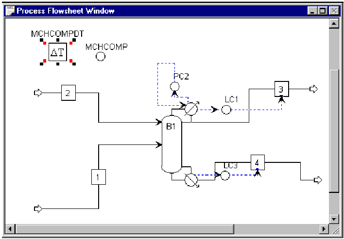
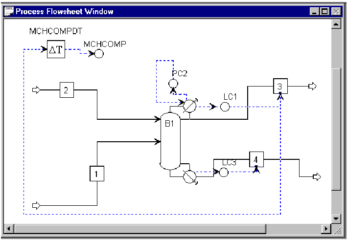
Наша схема выглядит следующим образом:

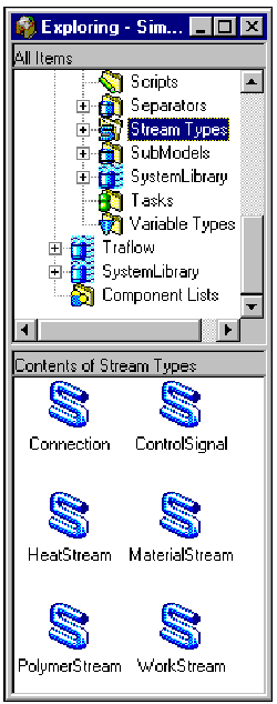
1. В библиотеке Dynamics, выбираем Типы потоков (Stream Types).

2. Выбираем объектControlSignalиудерживая кнопку мыши на иконке перетаскиваем его в окно технологической схемы. На схеме появляются стрелочки у портов, к которым можно подсоединиться.

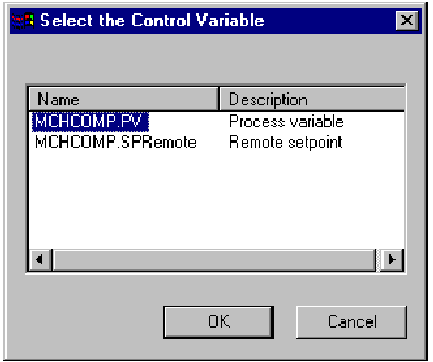
3. Переместим указатель мыши на поток 3, и отпустим кнопку мыши на порт, помеченный OutputSignal. Появляется диалоговое окно выбора управляющей переменной для потока 3.

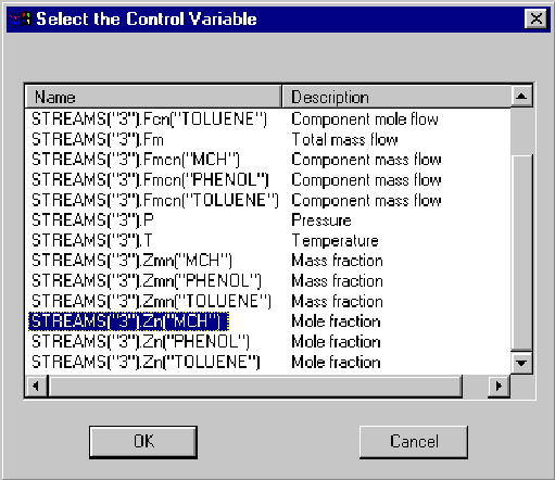
4. Выбираем Streams ("3"). Zn ("MCH"), затем нажимаем кнопку ОК.

5.В окне технологической схемы, курсор становится стрелкой подводим ее к блоку MCHCOMPDTна вход.

6.Снова выбираем объект ControlSignalиудерживая кнопку мыши на иконке перетаскиваем его в окно технологической схемы.

7. Отпустим кнопку мыши на выход блока MCHCOMPDT. Управляющий сигнал автоматически создан и готов к подключению.

8.Подведем стрелочку к блоку MCHCOMP, щелкним порт, помеченный InputSignal для подключения управляющего сигнала. Выбор управляющей переменной диалоговое окно:

Наша Технологическая схема выглядит так:

Указание манипулируемой переменной:

1. Выбираем объект ControlSignalиудерживая кнопку мыши на иконке перетаскиваем его в окно технологической схемы и подключим к выходу блока MCHCOMP.

2. Переместим указатель на вход потока-2.

Диалоговое окно выбора управляющей переменной:

3. Нажмем кнопку ОК.

Наша Технологическая схема выглядит так:

Т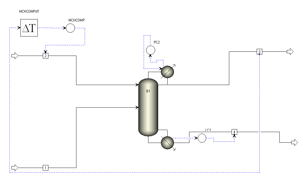еперь мы можем изменять настройкиPID-контроллера, для этого:

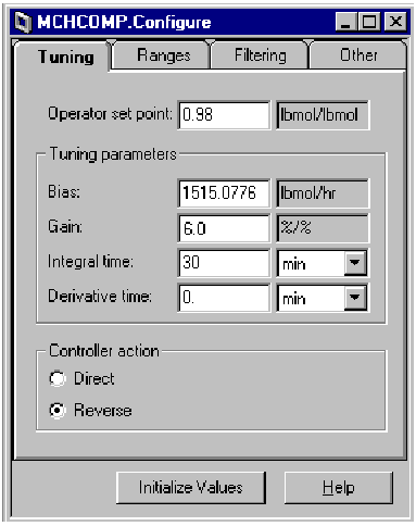
1. В окне технологической схемы, выбираем MCHCOMP.

2. Щелкнем правой кнопкой мыши на блоке. В появившемся списке выбираем Form → Configuration.

3. Появляется диалоговое окно

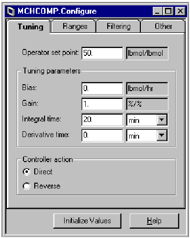
4. Нажмем кнопку InitializeValues.

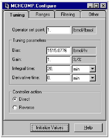
5. Контроллер MCHCOMP должен быть обратного действия, поэтому ставим флажок на Reverse.

6. Значение setpointустанавливаем 0,98.

7. Коэффициент усиления 6.

8. Время интегрирования 30 минут. Настройка вкладки теперь выглядит следующим образом:

Изменение диапазонов для процесса:

1. Щелкнем вкладку диапазонов.

2. Минимум устанавливаем 0,9.

3. Максимум устанавливаем 1.

4. Выходной диапазон значений без изменений. Вкладка Диапазоны теперь выглядит следующим образом:

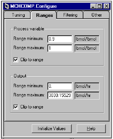
5. Нажмем кнопку «Закрыть», чтобы закрыть диалоговое окно.

Мониторинг Моделирования

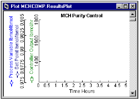
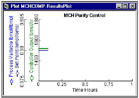
Открытие графика MCHCOMP контроллера

1. В технологической схеме, нажмем кнопку блока MCHCOMP, чтобы выбрать его, затем щелкнем правой кнопкой мыши.

2. Из меню, которое появляется, выбираем пункт Forms →ResultsPlot.Появляется график: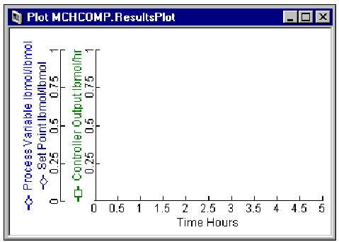

3. Расположим наши окна, чтобы можно было видеть график и схему.

Открытие лицевой панели MCHCOMP контроллераЛицевая панель показывает текущие значения переменных контроллера Set Point, Process Variable и Output during a simulation. Также можно использовать лицевую панель для изменения настроек контроллера.

1. В технологической схеме, дважды щелкнем на блоке MCHCOMP, появляется лицевая панель.

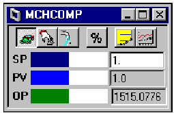
2. Расположим наши окна, чтобы можно было видеть график и схему илицевую панель.

Настройка графика.

1. Щелкнем в пустую область в пределах графика, а затем нажмем правую кнопку мыши.

2. В появившемся меню выберем пункт Properties.

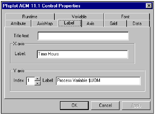
3. Щелкнем на вкладку Labels.

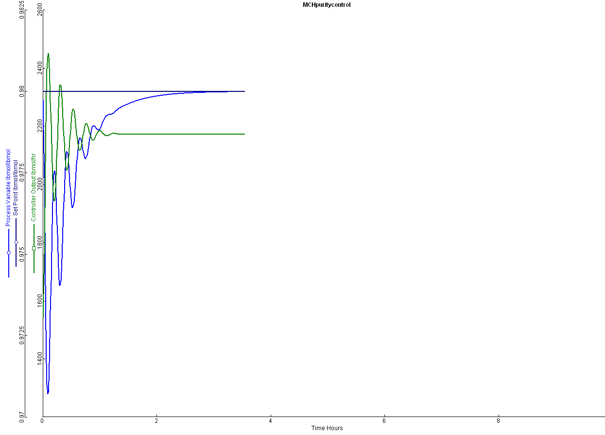
4. В поле Title Textвводим имя нашего графика: MCHPurity Control.

Настройка осей графика.

1. На графике, дважды щелкнем на номера на оси для настройки диапазона, появляется диалоговое окно.

2. В поле Axis Range, вводим диапазон от 0,975 до 0,985.

3. Нажимаем кнопку «OK», чтобы принять изменения. Чтобы изменить масштаб оси выхода контроллера:

1. На графике, дважды щелкнем на номера на оси выхода контроллера для настройки диапазона, появляется диалоговое окно.

2. Изменяем шаг (Grid Interval) на 200, затем в полеAxis Range вводим диапазон от 1200 до 1800.

3. Нажимаем кнопку «OK», чтобы принять изменения.

Открытие таблицы Манипулирования.

В таблице Манипулирование отображаются переменные, которые мы можем изменять вручную во время динамического моделирования.

1. В технологической схеме, выберем Stream 1, затем нажмем правой кнопкой мыши.

2. Из меню появляется Forms → Manipulate.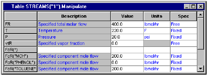

Теперь все готово для запуска моделирования.

Устанавливаем Pause Time:

1. Из меню Run, выбираем Pause At, отображаетсядиалоговое окно.

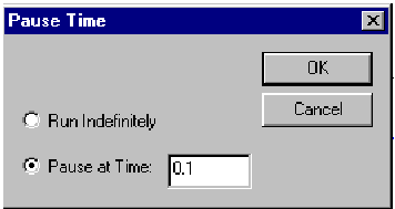
2. В диалоговом окне паузы, выбираем Pause at Timeи вводим значение 0,1.

3. Нажимаем «ОК» чтобы принять изменения.

4. На панели инструментов Run Control toolbar, нажимаем кнопкуRun, чтобы начать моделирование.

Теперь можно поменять температуру, давление или потоки компонентов.

и меняя Pause at Timeможно посмотреть, как происходит переходный процесс, а также менять настройки регулятора.

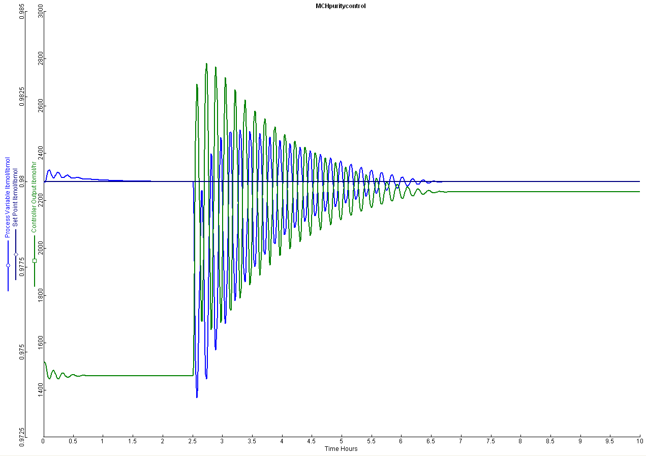
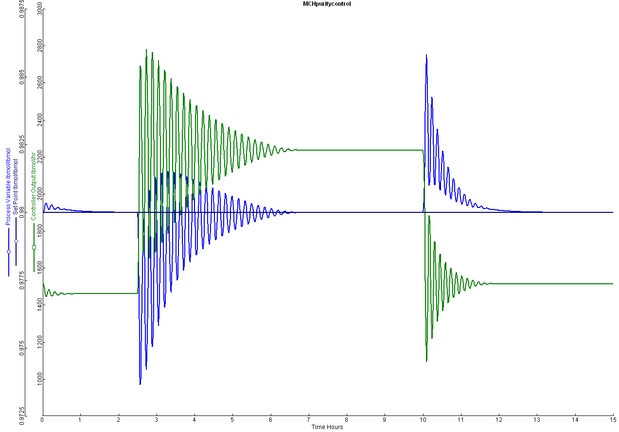
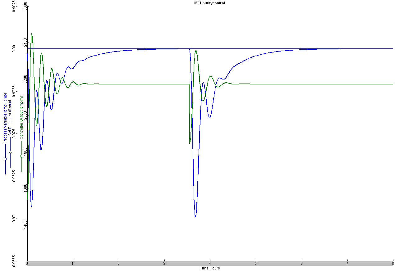
интегральная часть 10, пропорциональная 1,5

интегральная часть 15, пропорциональная 3

Вариант лекций на английском языке

Начало формы

1.Introduction. Modeling facilities and management systems. To model the facilities management along with systems needed to develop mathematical model not only for individual process units, and their control systems, as well as models of objects embedded in the flow charts. This is because the design of the controls necessary to consider not only individual objects but also their combination, which would take into account, the mutual influence of individual objects at each other, but also for your entire technological scheme as a whole. To solve such problems developed software packages that enable capacity-vat mathematical models of technological schemes, to carry out calculations of the steady-state aggregate processing facilities, combined with material and energy flows, often with recycle streams. In addition to the calculations of stationary modes are software-complex can simulate the work flow diagrams and in dynamic modes. At the same time in such a simulation can also consider the impact on work patterns of regulatory systems of individual process parameters and create the optimal management of individual systems Ob-ektami and schemes as a whole, taking into account the mutual influence of technological facilities to test the quality of operation of the facility management. In this case, the criterion function can be used as a criterion to use for quality control of individual devices flowsheet and test the quality of functioning of the whole process. To solve such problems created by various software packages nye. These various programs contain a set of routines that enable the following tasks necessary for the simulation of flow diagrams and control systems.

 

Н

1. Bank data on the properties of individual components of mixtures involved in the processes. 2. System simulation of the mixture on the properties of the components that make up the technological flow, taking into account the dependence of the properties of individual components of the temperature and-pressure. 3. Bank of technological facilities, which may consist of flow chart and their models. Such models can convert input process streams at the weekend. 4. Bank of different genera fittings, acting on the process streams. 5. Bank of instrumentation and actuators to ensure impact of the process streams and for providing measurement and maintenance of specified levels of process parameters. 6. System for calculating a set of mathematical models of technological facilities with regard to their relations and recycle streams. The system usually provides a break at the beginning of new relationships recycle, followed by iterative calculations to ensure convergence of the dangling bonds on all components of process streams. 7. System optimization of manufacturing facilities and schemes formulated by the criterion of optimization and set parameters to vary. We will consider the problem of modeling technological objects and control systems of software system using ASPEN, developed by Hyprotech. This is the most widely used to model complex flowsheets in various fields of technology. Bank data on the properties of individual components and a set of technological objects and their models can solve the problem of simulating circuits and control systems for various industries for chemical industry, chemical and pharmaceutical industries, the production processes of mineral fertilizers, for refining of the processes and petrochemicals for the production of polymers for steel of production, including pyrometallurgical processes and hydrometallurgical processes. Ability to work with this software system provides a wide range of components in a database on the properties of components and a wide range of process modules and their mathematical models. The possibility of using this system is ensured by the fact that both the bank - a bank of data on physico-chemical properties and bank models of technological facilities are open banks. And can be supplemented by the introduction of additional properties of the components for which there is data in the bank and the creation of so-called user models

 

If it becomes necessary to use non-standard models, which are absent in the library-tech models. When you create a mathematical model of technological scheme and control systems must perform the following typical steps that are characteristic of this work, using any software package. 1. Create a flow chart of control object. To do this, select the appropriate template technological schemes to choose from a library of objects relevant technological modules and place them on the field of the technologically scheme. 2. Connect all the objects in the form of technological streams of material and energy flows. 3. Determine the composition of each stream. 4. Specify the required values ​​of technological parameters of each technological unit. 5. Save the model generated the technological object. 6. Go to the subsystem, which provides simulation of dynamic modes of the scheme. 7. Call the subsystem model generated flowsheet. 8. Supplement scheme measuring devices and control of individual process parameters. 9. Conduct a simulation of the created scheme. 10. Enter into the subsystem optimization to formulate a criterion of optimization, to determine the parameters of the optimization, the variation intervals, select the optimization method to solve the problem and optimizing the. Consider the solution of these problems by using software package Aspen. You need to log in Aspen, enter the subsystem Aspen plus and enter into the main window of the system.

What is an Aspen Plus Process

Simulation Model?

A process consists of chemical components being mixed, separated, heated, cooled, and converted by unit operations. These components are transferred from unit to unit through process

streams. You can translate a process into an Aspen Plus process simulation model by performing the following steps:

1 Define the process flowsheet:

Define the unit operations in the process.

Define the process streams that flow to and from the unit operations.

Select models from the Aspen Plus Model Library to describe each unit operation and place them on the process flowsheet.

Place labeled streams on the process flowsheet and connect them to the unit operation models.

2 Specify the chemical components in the process. You can take these components from the Aspen Plus databanks, or you can define them.

3 Specify thermodynamic models to represent the physical properties of the components and mixtures in the process.

These models are built into Aspen Plus.

4 Specify the component flow rates and the thermodynamic conditions (for example, temperature and pressure) of feed streams.

5 Specify the operating conditions for the unit operation models.

With Aspen Plus you can interactively change specifications such as, flowsheet configuration; operating conditions; and feed compositions, to run new cases and analyze process alternatives.

In addition to process simulation, Aspen Plus allows you to perform a wide range of other tasks such as estimating and regressing physical properties, generating custom graphical and

tabular output results, fitting plant data to simulation models, optimizing your process, and interfacing results to spreadsheets.

The Aspen Plus Main Window

When you start Aspen Plus, the main window appears. This window is similar to usual window of Windows and has several rows that allow to use all possibilities of Aspen Plus. Bellow we can see this main window and further we shall consider all features of this window.

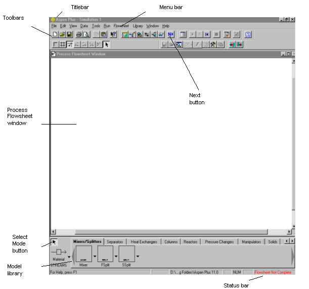
The upper row contains Title bar. In this bar is written Simulation 1 on default. After starting creating new task You can assign to your task any name. The second row is row for different commands, so called Menu bar. This bar contains different buttons for fulfillment of different action at creating new task and for edition existing tasks. Every button from this bar has special inner menu, which is opened after clicking on this button. Further we will consider every button in more details. Among of these buttons it should be noted the button “Next”. This buttons allows always to know to find out next action which must be made for creation new task.

The third row contains of the buttons for work during creation and edition of your technological scheme.

Use the workspace to create and display simulation flowsheets and PFD-style drawings. You can open other windows, such as Plot windows or Data Browser windows, from the Aspen Plus main

window.

Table 1. Description of main window of Aspen Plus/

Window Part	Description
Titlebar	Horizontal bar at top of window that displays the Run ID. Simulation 1 is the default ID until you give the run a name.
Menu bar	Horizontal bar below the titlebar. Gives the names of the available menus.
Toolbar	Horizontal bar below the menu bar. Contains buttons that, when clicked, perform commands.
Next button	Invokes the Aspen Plus expert system. Guides you through the steps required to complete your simulation.
Status bar	Displays status information about the current run.
Select Mode button	Turns off Insert mode for inserting objects, and returns you to Select mode.
Process Flowsheet window	Window where you construct the flowsheet
Model library	Area at the bottom of the main window. Lists available unit operation models.
Aspen Plus Toolbars	Use the buttons on the toolbars to perform actions quickly and easily.

The default toolbars are shown here:

For information on viewing different toolbars, see Viewing Toolbars.

The Process Flowsheet Window

The Process Flowsheet window is where you create and display simulation flowsheets and PFD-style drawings.

You can display the process flowsheet window in three different ways:

To display the Process Flowsheet window as	From the Window menu, click
A normal window	Normal
A window always in the background	Flowsheet as Wallpaper
A sheet of a workbook	Workbook mode

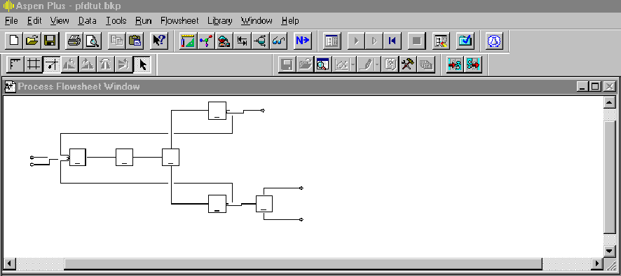
The Model Library

Use the Model Library to select unit operation models and icons that you want placed on the flowsheet. The Model Library appears at the bottom of the Aspen Plus main window.

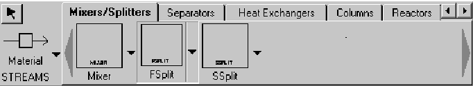
Selecting a Unit Operation Model from the Model Library

To select a unit operation model:

1 Click the tab that corresponds to the type of model you want to place in the flowsheet.

2 Click the unit operation model on the sheet.

3 To select a different icon for a model, click the down arrow next to the model icon to see alternate icons. The icon you select will appear for that model in the Model Library.

4 When you have selected a model, click location in the flowsheet where you want to place the model. When you place blocks this way, you are in Insert mode. Each time you click in the Process Flowsheet window, you place a block of the model type that you specified. To exit Insert mode and return to Select mode, click the Mode.

Selecting the Stream Type from the ModelLibrary

To select the stream type:

1 Click the down arrow next to the stream type displayed in the Model Library.

2 Select the stream type you want to place in the flowsheet.

3 Once a stream type is selected, simply click the ports on the flowsheet where you want to connect the stream.

When placing blocks and streams, the mouse pointer changes to the crosshair shape, indicating Insert Mode. After placing each block or stream, you remain in Insert Mode until you click the

Select Mode button in the upper right corner of the Model Library. For more information on what the mouse pointers mean, see Mouse Pointer Shapes.

For more details and examples for setting up a flowsheet, see Getting Started Building and Running a Process Model.

The Data Browser

The Data Browser is a sheet and form viewer with a hierarchical tree view of the available simulation input, results, and objects that have been defined.

To open the Data Browser:

Click the Data Browser button on the Data Browser toolbar.

– or –

From the Data menu, click Data Browser.

The Data Browser also appears when you open any form.

Use the Data Browser to:

Display forms and sheets and manipulate objects

View multiple forms and sheets without returning to the Data menu, for example, when checking Properties Parameters input

Edit the sheets that define the input for the flowsheet simulation

Check the status and contents of a run

See what results are available

The Parts of the Data Browser

The parts of the Data Browser window are:

Window Part	Description
Form	Displays sheets where you can enter data or view results
Menu Tree	Hierarchical tree of folders and forms
Status Bar	Displays status information about the current block, stream or other object
Prompt Area	Provides information to help you make choices or perform tasks
Go to a Different Folder	Enables you to select a folder or form to display.
Up One Level	Takes you up one level in the Menu Tree
Folder List	Folder List

Units	Shows units of measure used for the active form
Go Back button	Takes you to the previously viewed form
Go Forward button	Takes you to the form where you last chose the Go Back Button
Input/Results View Menu	Allows you to view folders and forms for Input only, Results only, or All
Previous Sheet button	Takes you to the previous input or result sheet for this object
Next Sheet button	Takes you to the next input or result sheet for this object
Comments button	Allows you to enter comments for a particular block, stream, or other object
Status button	Displays any messages generated during the last run related to a particular form
Next button	Invokes the Aspen Plus expert system. Guides you through the steps required to complete your simulation.

Displaying Forms and Sheets in the Data Browser.

Use the Data Browser to view and edit the forms and sheets that define the input and display the results for the flowsheet simulation. When you have a form displayed, you can view any sheet on the form by clicking on the tab for that sheet.

There are several ways to display forms. You can display a form in a new Data Browser by using:

The Data menu

Block or stream popup menus

The Check Results button on the Control Panel, the Check Results command from the Run menu, or the Check Results button on the Simulation Run toolbar.

The Setup, Components, Properties, Streams, or Blocks buttons on the Data Browser toolbar

The Next button on the Data Browser toolbar

The Data Browser button on the Data Browser toolbar You can move to a new form within the same data browser by using the:

Menu tree

Object Managers

Next button on the Data Browser

Previous Form and Next Form buttons (<<, >>)

Go Back and Go Forward buttons

Select View menu

Up One Level button

Status Indicators

Status indicators display the completion status for the entire simulation as well as for individual forms and sheets.

The status indicators appear:

Next to sheet names on the tabs of a form

As symbols representing forms in the Data Browser menu tree

This table shows the meaning of the symbols that appear:

This Symbol	On an	Means
	Input form	Required input complete
	Input form	Required input incomplete
	Input form	No data entered
	Mixed form	Input and Results
	Results form	No results present (calculations have not been run)
	Results form	Results available without Errors or Warnings (OK)
	Results form	Results available with Warnings
	Results form	Results available with Errors
	Results form	Results inconsistent with current input (input changed)

	Input folder	No data entered
	Input folder	Required input incomplete
	Input folder	Required input complete
	Results folder	No results present
	Results folder	Results available – OK
	Results folder	Results available with Warnings
	Results folder	Results available with Errors
	Results folder	Results inconsistent with current input (input changed)
	Beside folder or formEO input or results OK
	Beside folder or formEO input or results with Errors

A form is a collection of sheets