RM7

ISSN 1063-7397, Russian Microelectronics, 2006, Vol. 35, No. 1, pp. 7–20. © Pleiades Publishing, Inc., 2006.

Original Russian Text © A.Yu. Bogdanov, Yu.I. Bogdanov, K.A. Valiev, 2006, published in Mikroelektronika, 2006, Vol. 35, No. 1, pp. 11–26.

Schmidt Modes and Entanglement

in Continuous-Variable Quantum Systems

A. Yu. Bogdanov**, Yu. I. Bogdanov*, and K. A. Valiev*

*Institute of Physics and Technology, Russian Academy of Sciences, Moscow, Russia

e-mail: [e-mail]

**Moscow State University, Moscow, Russia

Received June 26, 2005

Abstract—The extraction of Schmidt modes for continuous-variable systems is considered. An algorithm based on the singular-value decomposition of a matrix is proposed. It is applied to the entanglement in (i) an atom–photon system with spontaneous emission and (ii) a system of biphotons with spontaneous parametric downconversion (SPDC) of type II. For the atom–photon system, the evolution of entangled states is found to be governed by a parameter approximately equal to the fine-structure constant times the atom-to-electron mass ratio. An analysis is made of the dynamics of atom–photon entanglement on the assumption that the system’s evolution is determined by the superposition of an initial and a final state. It is shown that in the course of emission the entanglement entropy first rises on a timescale of order the excited-state lifetime and then falls, approaching asymptotically a residual level due to the initial energy spread of the atomic packet (momentum spread squared). SPDC of type II is analyzed by means of the polarization density matrix and a newly introduced coherence parameter for two spatially separated modes. The loss of intermodal coherence is addressed that results from the difference in behavior between ordinaryand extraordinary-ray photons in a nonlinear crystal. The degree of intermodal coherence is investigated as a function of the product of crystal length and pump bandwidth.

DOI: 10.1134/S1063739706010021

1. INTRODUCTION

Schmidt decomposition is an effective tool for analyzing entangled quantum states [1]. Recently, entanglement has been examined in the context of continu- ous-variable systems [2–4]. It turns out that such systems can be effectively described by a manageable number of Schmidt modes in some situations of physical interest in spite of the infinite dimension of the quantum state space.

This paper presents a numerical analysis of entangled systems by the singular-value decomposition (SVD) of matrices. An SVD algorithm for the numerical extraction of Schmidt modes is proposed and applied to the entanglement in (i) an atom–photon system with spontaneous emission and (ii) a system of biphotons generated by spontaneous parametric downconversion (SPDC) of type II.

For the atom–photon system, we show for the first time that the evolution of entangled states is determined by a parameter of order the fine-structure constant times the mass ratio of the atom to an electron. We examine the dynamics of the system under emission, the evolving state being determined by the superposition of an initial and a final state. We demonstrate that entanglement develops between the atomic and photonic degrees of freedom on a timescale of order the

excited-state lifetime before decaying asymptotically to a low residual level related to the energy spread of the original atomic packet (momentum spread squared). For the first time, analytical expressions for the photonic modes are derived. The results obtained are interpreted in terms of the momentum representation.

SPDC of type II is investigated by means of the polarization density matrix and a newly introduced coherence parameter. For the first time, we address the development of intermodal decoherence resulting from the difference in behavior between an ordinary and an extraordinary photon in a nonlynear crystal. The degree of intermodal coherence is examined as a function of the product of crystal length and pump bandwidth. Examples of Schmidt-mode analysis are given for different degrees of coherence.

The paper is organized as follows. Section 2 provides background information on Schmidt decomposition and describes the SVD algorithm. A comparison is made between our algorithm and ones constructed by previous workers.

Section 3 deals with entangled states in an atom– photon system with spontaneous emission. We ascertain how the structure of Schmidt modes, the Schmidt number, and the entanglement entropy vary with the

7

8	BOGDANOV et al.

momentum spread of the atomic packet. We show that the system’s evolution is determined by a parameter made up of atomic constants, which is of order the finestructure constant times the mass ratio of the atom to an electron.

Section 4 examines the asymptotic behavior of the atom–radiation system in terms of the momentum representation. The discussion rests on the Weisskopf– Wigner theory of natural line width for a two-level atom, the theory being modified to include atomic recoil energy and the momentum distribution over an original packet.

Section 5 is concerned with SPDC, in which a pump photon is converted into two photons each of which has about half the energy of the original photon. Such systems manifest entangled spectral and polarization properties when produced by SPDC of type II with pump pulses 10–100 fs wide, in which case as-created photons are polarized in two mutually orthogonal directions.

Section 6 analyzes SPDC of type II by means of the polarization density matrix and a newly introduced coherence parameter for two spatially separated modes. The degree of intermodal coherence is investigated as a function of the product of crystal length and pump bandwidth.

Section 7 presents the main conclusions of this study.

2. SCHMIDT DECOMPOSITION AND THE SVD ALGORITHM

Let the probability amplitude (wave function) ψ(p, q) of the system be a function of two continuous variables p and q. For computational purposes, it is rep-

resented	in discrete form as a matrix
ψ j1 j2 =	ψ ( p j1, q j2 ), where 1 ≤ j1 ≤ n, 1 ≤ j2 ≤ n.

Assume that the probability amplitude is defined on an n × n uniform grid. Our computations have shown that the computed values change little with n if this is large enough. The results presented below are obtained at n in the range 300–800, but it is sufficient to set n to

30–50 in most of the examples.
The Schmidt	decomposition [1] of a	matrix
ψ ( p j1, q j2 ) is defined by
	n
ψ ( p j1, q j2 ) =	∑ λk ψk(1)( p j1 )ψk(2)( q j2 ),	(1)

k = 1

where λk are weighting coefficients satisfying the normalization condition

∑λk = 1.	(2)
k

We arrange the right-hand terms of Eq. (1) in descending (nonascending) order of λk.

ψ(1) ψ(2)

The functions k (p) and k (q) are termed

Schmidt modes. Although there are in general n modes of each type (the total number growing idefinitely with n), the first few modes are sufficient in many situations of physical interest, the sum of their weighting coefficients being close to 1. In terms of calculation, this means that we can change from an infinite-dimensional Hilbert space to one of manageable dimension.

If more than the first right-hand term are important in Eq. (1), the degrees of freedom corresponding to p and q are entangled. This implies, among other tfind-

ψ(1)

ing p in the state k (p) means finding q in the state ψ(k2) (q) (with the same k).

In what follows, we shall use some quantities characterizing the effective number of modes involved in a Schmidt decomposition. A first characteristic, the

Schmidt number, is defined by
K	=	1	(3)
		------------,
		∑λk2

k

where λk are as in Eq. (1) [2]. Note that K is not less than unity, due to condition (2) (K = 1 only if the Schmidt decomposition has a unique nonzero term).

As a second characteristic, we take the well-known

entanglement entropy
S = –∑λk log2λk ,	(4)
k

which is always nonnegative (and is 0 only if the Schmidt decomposition has a unique nonzero term) [1].

The Schmidt decomposition of a probability amplitude is a far more compact expansion than the double Fourier series with respect to any given set of orthogonal functions. Changing to a Schmidt decomposition is effectively passing to a diagonal representation of the Fourier-coefficient matrix (which may be a square matrix). However, Schmidt modes are specific to the physical system considered.

We now describe our algorithm for the numerical extraction of Schmidt modes. By ψ we denote an n × n

probability-amplitude matrix, and by ψ j1 j2	its ele-
ments. We then introduce the matrix
M = ψψ+.	(5)
Having found the eigenvectors and eigenvalues of M,
we arrive at the expansion
M = UDU+.	(6)

RUSSIAN MICROELECTRONICS Vol. 35 No. 1 2006

SCHMIDT MODES AND ENTANGLEMENT

9

Here, U is a unitary matrix having the eigenvectors of M as its columns, and D is a diagonal matrix in which the leading diagonal consists of the eigenvalues λk of M arranged in descending (nonascending) order.

In fact, the leading-diagonal elements of D are the weighting coefficients λk of the Schmidt decomposition,

ψ(1)

and the mode k (p) is given by the kth column of U.

ψ(2)

To find the modes k (q), we introduce the matrix

V = D–1U+ψ .

(7)

In cases of high dimensionality, some of the lead- ing-diagonal elements of D may be so close to zero as to make D–1 difficult to compute with adequate accuracy (zero-divide problem). This situation can be avoided in two equivalent ways. One of them is to perturb such elements by reasonable amounts (e.g., of order 10–16–10–12). The other way is to change from D to its reduced version whose leading diagonal consists of elements of adequate magnitude, λ1, λ2, …, λr (this implies rejecting the columns of U other than the first r columns).

ψ(2)

The kth row of V constitutes the mode k (q).

Using the matrices U and V, we obtain the following expansion of ψ:

ψ = USV ,

(8)

where S = D is a diagonal matrix in which nonneg-

ative leading-diagonal elements, λk , are arranged in descending (nonascending) order. Expansion (8) is the SVD of the matrix ψ, and λk are the singular values ψ.

The algorithm presented highlights the self-consis- tent nature of Schmidt-mode extraction with respect to p and q. This means, among other things, that every col-

ψ(1)

umn of U (every mode k (p)) is computed up to an insignificant complex factor of unit modulus; if this fac-

ψ(2)

tor is included, the phase of the mode k (q) will change accordingly (see Eq. (7)), the mode being

entangled with the original mode.

We see some advantages in the above algorithm over previously reported ones [3, 4].

Law et al. [3] proposed that Schmidt modes be derived from two independent (and uncoupled) equations [3, Eqs. (3) and (4)]. However, their approach ignores the self-consistent nature of the problem and therefore can be misleading. An example is the fact that the entangled variables corresponding to modes 3 and 4 of Fig. 2 were incorrectly found to have a relative phase of π [3].

Lamata and Leon [4] followed an overly complex procedure whereby the probability amplitude as a function of two variables is expanded in a double Fourier series in terms of Hermite functions before extracting Schmidt modes. Furthermore, such a treatment requires a large number of basis functions for the results to be accurate.

3. ENTANGLED STATES

OF AN ATOM–PHOTON SYSTEM WITH SPONTANEOUS EMISSION

Consider a confined two-level atom that is made to pass from the ground state represented by a one-dimen- sional Gaussian wave packet (as with the harmonic oscillator) to the excited state by means of a laser pulse applied at the instant t = 0. The pulse is assumed to be much shorter than the excited-state lifetime; this is equal to 1/γ, where γ is the excited-level width measured in frequency units. The confining field is assumed to be turned off at t = 0, so that the atom–photon system is free from external influence at times following this instant.

The states of an atom–photon system with spontaneous emission are rigorously treated within the quantum theory of radiation [5]. We shall deal with this topic in a heuristic manner.

Let the atom and the photon travel along the same straight line in opposite directions. Then the probability amplitude of the atom–photon system can be written

			1			2	( p + q)	2
ψ ( p, q)	= θ( τ – p) exp				exp –	η				.	(9)
			–--	( τ – p)		---------------------------------
			2			2( 1 + τη2ξ0i)

with coordinate-independent factors being left out. Equation (9) is valid for τ 1, where τ = γt is dimensionless time. It involves these quantites:

rphγ

p = ---------

c

is the dimensionless photon coordinate as measured with a detector and

ratγ

q = --------

νrec

is the dimensionless atom coordinate, for which νrec is the atom recoil speed given by

RUSSIAN MICROELECTRONICS Vol. 35 No. 1 2006

10	BOGDANOV et al.

ν ω rec = -------

Mc

with ω, M, and c being the transition frequency, atom mass, and speed of light, respectively. The variables rph and rat and hence p and q may be positive or negative.

Further,

	η =	νrec	=	ω
		γ-------a0		----------------Mcγ a0

is a dimensionless quantity related to the initial width a0 of the Gaussian wave packet (a0 is measured in length units).

Since η varies inversely as a0, it is proportional to the initial momentum spread (due to the uncertainty principle). Accordingly, we call η the momentumspread parameter. A similar parameter was introduced by Chan et al. [2].

The initial state of the atom is represented by

ψ ( rat, t = 0)		rat2	(10)
	= const exp	–------- .
		2a2
		0

This implies that the coordinate distribution has variance a20 /2.

The quantity

ξMc2 γ

=------------

0 ω ω

is a dimensionless constant dependent on the properties of the atom only.

Finally, i = –1 .

Equation (9) allows of a simple physical interpretation.

The first right-hand factor, the Heaviside unit-step function, indicates that the probability amplitude is exactly zero at all p > τ, i.e., at points that the photon cannot reach within the time τ.

The second factor represents the exponential decay of the probability amplitude of emission from the excited state, for it involves the excited-level width γ [6].

The third factor is responsible for entanglement and can be interpreted as follows. The atom and the emitted photon constitute a system described by probability amplitude (9) throughout the period from the initial instant to a detection instant τ. The motion of the system’s center of inertia corresponds to the free motion of the Gaussian packet, which broadens with time. In other words, the law of conservation of momentum implies that the center of inertia behaves as a freely moving quantum “particle” until the system is perturbed (by detection of the photon or the atom).

The coordinate rci of the center of inertia can be characterized by the dimensionless quantity p + q. To see this, note that, in one-dimensional approximation,

rph = rci + ct, rat = rci – νrect ,

since the photon and the atom move in opposite directions. Hence,

p + q	rphγ ratγ			= rciγ	1	1	rciγ	(11)
	= ---------	+	--------νrec		-- +	-------ν rec	≈ --------.
	c				c		νrec

It can be shown that a freely broadening Gaussian packet can be represented by the third right-hand factor in Eq. (9) [7].

The uncertainty in the position of the center of inertia is inherent in an atom–photon system. If the packet is narrow at an initial instant (a0 small), it will broaden rapidly due to the uncertainty principle. In other words, a high degree of certainty for an initial coordinate of the center of inertia implies a low degree of certainty for an initial momentum, which makes the position of the center of inertia far less certain at later instants.

It can be shown that there is an optimum value of a0 such that the amount of broadening at the detection instant τ is minimal. The corresponding optimum value of η is given by

ηopt =	1
	-----------
	ξ0	τ .	(12)

The parameter

ξMc2 γ

=------------

0 ω ω

governs the evolution of entangled states. Notice that it

is given by the product of the large quantity	Mc2
	---------
	ω

(Mc2 = atomic energy, ω = photon energy) and the

small quantity	γ	the dipole approximation		the
	--- . In
	ω
quantum theory of radiation [6] yields the estimate
ξ0 =	Mc2 γ	αM	M
	------------	--------	-------------	(13)
	hω ω	m	= 137m,

where m is the electron mass, M is the atom mass, and

α1

=-------- is the fine-structure constant. 137

We see that ξ0 is large (ξ0 > 10), because even a hydrogen atom is about 2000 times as heavy as an electron.

RUSSIAN MICROELECTRONICS Vol. 35 No. 1 2006

SCHMIDT MODES AND ENTANGLEMENT

	The amount of packet broadening that accompanies	Consequently,
	the emission is assumed to be small. It follows that with
	the emission time
	1
	t --
	γ	By definition,
	the diffusion quantum length

η1

----.

ξ0

11

(15)

ht	h
----	-------
M	Mγ

is small compared with a0 [5]. We thus arrive at the condition

η	1
	--------
	ξ0 .	(14)

a0	=	1	,
----		--------
λ		ξ0η

so that conditions (14) and (15) can be recast as

1	a0	1.	(16)
--------	----
ξ0	λ

Condition (14) combined with estimate (13) imply that η is at most of order 0.1. This finding casts doubt on the physical significance of the values η = 10 to 1000 taken in [2, 8].

On the other hand, η is also bounded below. A small η implies a large a0, leading to loss of coherence between the photon being emitted and the atomic oscil-

lator. With a large a0, the phase factor exp(ik r ) is

close to zero (k = photon wave vector, r = oscillator position vector). The requirement of photon–oscillator coherence means a0 being small compared with the wavelength

Relation (16) identifies the range of validity for the theory presented. In particular, a0 must lie within a fairly narrow interval.

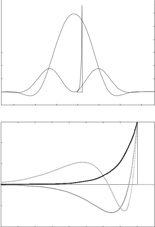
Figure 1a gives an example of the joint probability amplitude of an atom–photon system (the first Schmidt

mode is shown) calculated for ξ0 = 100, η = 0.03, and

τ = 10. Notice high uncertainty in the atomic coordinate (even the direction of recoil cannot be predicted unambiguously).

Figure 1b displays the first three Schmidt modes of radiation (mode 0 accounts for most of the total weight).

Schmidt modes can be approximated to a high accu- λ = λ/( 2π ). racy by a set of orthogonal functions based on Laguerre

polynomials:

(1)		1
ψk ( p)	= Ck Lk ( τ – p) exp –	--	( τ
		2

where Ck are normalizing constants.

In Fig. 1b the Schmidt modes evaluated numerically (data points) virtually coincide with those obtained by analytical approximation (solid lines), the relative accuracy of the latter being of order 10–3. The numerical evaluation was made at n = 800.

In the Weisskopf–Wigner model, the dynamics of an atom–photon system during emission is qualitatively determined by the superposition of an initial and a final state [6, 9]. The weight of the initial state |e |0 (an excited atom and no photons) decreases with time:

	θ( τ – p) ( k = 0, 1, … ),	(17)
– p)

λ(e)( t) = exp( –γt).

That of the final state |g |1 (a ground-state atom and one photon) grows:

λ(g)( t) = 1 – exp( –γt).

It follows from the above that, disregarding the fine structure of state (9), the Schmidt number and the entanglement entropy are given by

K0( t) =		1
	--------------------------------------------------		,	(18)
	( λ(e)( t) )2	+ ( λ(g)( t) )2

RUSSIAN MICROELECTRONICS Vol. 35 No. 1 2006

12								BOGDANOV et al.
Ψ								ξ0 = 100, τ = 10, η = 0.03
0.14
								(a)
0.12
0.10
0.08								Photon
						Real part

0.06
0.04
0.02	Imaginary
		part
0
–0.02	–150	–100	–50	0		50	100	150
				p(q)
Ψ		lam0 = 0.99955, lam1 = 0.0004486, lam2 = 4.01 Â – 7
0.15
				(b)
0.10
							Mode 0
0.05
0
				Mode 1
– 0.05								Mode 2
– 0.10	– 4	– 2	0	2	4	6	8	10	12
– 6
				p

Fig. 1. (a) Example of the joint probability amplitude for an atom–photon system (the first Schmidt mode is shown) and (b) the first three Schmidt modes of radiation. The data points and solid curves refer to numerical and analytical evaluation, respectively. The graphs are plotted for ξ0 = 100, η = 0.03, and τ = 10.

RUSSIAN MICROELECTRONICS Vol. 35 No. 1 2006

	2.0
	1.8
	1.6
	1.4
	1.2
K(S)	1.0
	0.8
	0.6

0.4

0.2

0

6 × 10–3

		5
	)	4
	0
	-S
	(S
	0	3
	-K
	K
		2
		1
		0

SCHMIDT MODES AND ENTANGLEMENT

13

(a)

K

S

2	4	6	8	10	12
		τ	η = 0.03
		ξ0 = 100,

(b)

S-S0

K-K0

2	4	6	8	10	12
		τ

Fig. 2. Calculating the dynamics of the Schmidt number and the entanglement entropy. In panel (a) the data points and solid curves refer to numerical evaluation and to analytical evaluation disregarding the fine structure of state (9), respectively, the curves being based on the Weisskopf–Wigner theory (Eqs. (18) and (19)). Panel (b) shows the time-dependent difference between the values of each characteristic obtained by the two approaches.

S0( t) = – ( λ(e)( t) )2log2{ ( λ(e)( t) )2 } – ( λ(g)( t) )2log2{ ( λ(g)( t) )2 }.		(19)

Figure 2a depicts the dynamics of the Schmidt number and the entanglement entropy as predicted by numerical evaluation (data points) or the Weisskopf– Wigner theory (solid curves). It is seen that evaluation with regard for the fine structure of state (9) (data

points) yields almost the same result as analytical evaluation by Eqs. (18) and (19) (solid curves). The graphs also indicate that in the course of emission the atomic and photonic degrees of freedom become entangled on

a timescale τ < 1, the entanglement vanishing at τ 1.

RUSSIAN MICROELECTRONICS Vol. 35 No. 1 2006

14	BOGDANOV et al.

Figure 2b shows the time-dependent difference between the values of each characteristic obtained by numerical and analytical evaluation, K(t) – K0(t) and S(t) –

S0(t) (vertical scale factor 10–3). In the limit τ 1, we have

		K∞ ≈ 1 + η2,				(20)
η2		ln	1	+ 0.5(		(21)
S∞ ≈ -------			---		1 + ln2) ,
ln2			η

where η 1.

We see that the residual entanglement as given by Eqs. (20) and (21) is governed by the initial energy spread (momentum spread squared).

It is convenient to treat the asymptotic properties of an atom–photon system in the momentum representation. This will be done in the next section.

4. SPONTANEOUS EMISSION

IN THE MOMENTUM REPRESENTATION

In the Weisskopf–Wigner theory, the natural line width of a two-level atom is derived from the formula

a( ωph )	1
	----------------------------------		,	(22)
	ωph – ω	+ iγ /2

where a(ωph) is the probability amplitude; ω and γ are the frequency and width of the atomic transition, respectively; and ωph is the photon frequency [6, 9].

We modify this formula to include the initial momentum distribution over the atomic packet and the emission recoil energy:

				p 2 a2
		exp –		----------a 0
				2	h	2	(23)
Ψ( ωph, pa ) = C------------------------------------------------------------------------.
		p a		γ
ωph	1 –	-------Mc	+ -------	2 ξ 0 – ω + iγ /2

The numerator is the amplitude of the packet in the momentum representation (the Fourier transform of

expression (10)). In the denominator the terms 1 –

pa		γ
-------		and ------- represent the frequency shifts due to the
Mc		2ξ0

Doppler effect and the recoil, respectively. Also, C is a normalizing coefficient.

Equation (23) applies at t 1/γ, when the weight of the initial state is close to zero (as with Eq. (9)). It also assumes that the packet changes little during the emission time, 1/γ, leading to the condition η 1.

We now introduce the dimensionless photon frequency νph and the dimensionless atom momentum πa:

		πa2
	exp	–----2	(26)
Ψ( νph, πa ) = C--------------------------------------------------.
νph +	-------1 – ηπa + i/2
	2ξ0

Since η 1 and ξ0 1, the denominator of Eq. (26) is close to that of formula (22), so that state (26) is approximated by the product of Lorentzian photonic factor (22) and the Gaussian atomic factor, implying a small amount of entanglement between νph and πa. Equations (20) and (21) apply again, as supported by numerical calculation.

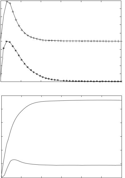
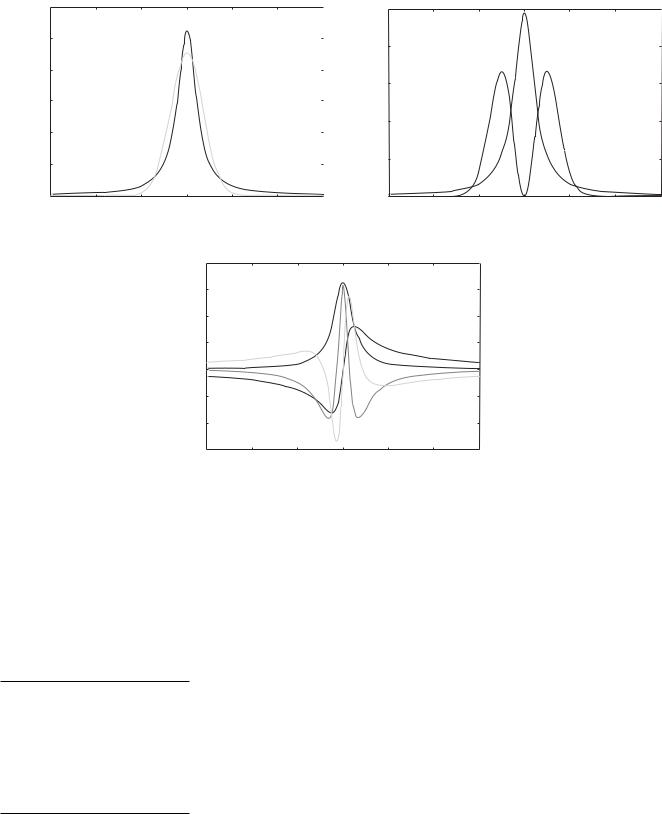
Figure 3 displays the first two Schmidt modes. Panels 3a and 3b represent probabilities (amplitude modulus squared). Panel 3c gives a detailed picture of the first two photonic modes (real and imaginary parts).

ωph – ω	,	(24)	5. SPONTANEOUS PARAMETRIC
νph = -----------------
γ			DOWNCONVERSION

πa =	paa0
	----------	.	(25)
	h

In this case, νph is the same as the dimensionless photon momentum.

As a result, Eq. (23) becomes

SPDC is a nonlinear optical phenomenon in which a photon is converted into two ones whose frequencies make that of the original photon if the process occurs under static conditions [10]. If the resulting photons are polarized identically, the process is said to be type-I SPDC. If they are polarized in mutually orthogonal directions, one has type-II SPDC.

Let us consider type-II SPDC. In this case, the two photons can be associated with an ordinary and an

RUSSIAN MICROELECTRONICS Vol. 35 No. 1 2006

0.030

0.025

0.020

P 0.015

0.010

0.005

–6

				SCHMIDT MODES AND ENTANGLEMENT										15
		Mode 0, ξ0 = 100, η = 0.03						0.025		Mode 1, ξ = 100, γ = 0.03
		(a)		Photon						(b)
								0.020				Photon
								0.015				Atom
								P
				Atom				0.001
								0.005
								0	– 4	–2	0	2	4	6
	– 4	–2	0	2	4	6
								–6
	Photon frequency (atom momentum)								Photon frequency (atom momentum)

ξ0 = 100, η = 0.03

0.20

(c)

0.15

0.10		Mode 0, real part			Mode 0,
0.05	Mode 1,				imaginary part
Ψ	imaginary part
0
– 0.05					Mode 1,
					real part
– 0.10
– 0.15 –6		– 4	–2	0	2	4	6
			Photon frequency

Fig. 3. (a, b) The first two Schmidt modes in terms of probability (amplitude modulus squared) and (c) the first two photonic modes (real and imaginary parts of amplitude).

extraordinary ray, respectively, in the nonlinear crystal. We focus on a degenerate case where resulting photons have almost equal frequencies, half the pump frequency. The difference in behavior between an ordinary and an extraordinary ray leads to a distinction between the photons. The phenomenon concerned is very important with short pump pulses (10–100 fs), whose

bandwidth (1013–1014 Hz) is comparable with that of SPDC.

Assume that the three photons travel in the same direction. It has been shown that the probability amplitude ψ(ωo, ωe) of the creation of a pair of photons with respective frequencies ωo (ordinary ray) and ωe (extraordinary ray) can be written

ψ ( ωo, ωe ) = Cα( ωo, ωe )Φ( ωo, ωe ),	(27)

where

	( ωo + ωe	– 2ω )2	(28)
α( ωo, ωe ) = exp –	--------------------------------------σ2	,

RUSSIAN MICROELECTRONICS Vol. 35 No. 1 2006

16					BOGDANOV et al.
						L
	sin			( ko( ωo ) + ke( ωe ) – kp( ωo + ωe ) )
						--
Φ( ωo, ωe ) =						2
					----------------------------------------------------------------------------------------------				,	(29)
					L
			( ko( ωo ) + ke( ωe ) – kp( ωo + ωe ) ) --
			2

assuming that the pump spectrum is Gaussian [11– 13]. Here, C is a normalizing factor.

The term α(ωo, ωe) is determined by the pump spectrum. The parameters 2 ω and σ characterize the mean pump frequency and the pump bandwidth, respectively. Note that the pump frequency distribution (determined by α2) has variance σ2/4.

The term Φ(ωo, ωe) is governed by the properties of the crystal: its length L and its dispersion relations ko(ωo), ke(ωe), and kp(ωo + ωe) for the ordinary, extraordinary, and pump wave, respectively.

If ωo and ωe are close to ω , the following approximation can be used [11, 12]:

							L
	sin			( ( ωo – ω )( ko' – kp' ) + ( ωe – ω )( ke' – kp' ) )
							--
Φ( ωo, ωe )							2
	=				---------------------------------------------------------------------------------------------------------------					.	(30)
					L
			( ( ωo – ω )( ko' – kp' ) + ( ωe – ω )( ke' – kp' ) ) --
		2

Here the reciprocal group velocities are involved:

ko' =

∂ko( ω )

ke' =

∂ke( ω )

kp' =

∂kp( ω )

.

(31)

∂ω

ω = ω

∂ω

ω = ω

∂ω

ω = 2ω

To facilitate calculation, we measure bandwidth in

reciprocal picoseconds, σ being of order 10–100 ps–1. Likewise, a reciprocal-group-velocity difference times the crystal length is expressed in picoseconds. In Section 6 we

shall use the following typical experimental values: ( k'p –

k'e )L = 0.266 ps, ( k'p – k'o )L = 0.076 ps, and L = 1 mm [3]. Introducing the dimensionless quantities

p =	ω---------------o – ω	,	q =	---------------ωe – ω	,	(32)
	σ			σ
Xo = ( kp' – ko' ) Lσ,			Xe	= ( kp' – ke' ) Lσ		(33)

we express the SPDC probability amplitude in the compact form

2	sin[ 0.5( Xo p + Xeq) ]
ψ ( ωo, ωe ) = C exp( –( p + q) )	--------------------------------------------------		(34)
	[ 0.5( Xo p + Xeq) ] .

6. BIPHOTON COHERENCE

Let us consider a biphotonic field (created with, e.g., a beam splitter) consisting of two distinct spatial modes called the signal mode and the idler mode.

A biphotonic state vector produced by type-II SPDC includes frequency and polarization degrees of freedom. If the ordinary and the extraordinary ray are polarized horizontally and vertically, respectively, the state vector is written

RUSSIAN MICROELECTRONICS Vol. 35 No. 1 2006