Understanding the Human Machine - A Primer for Bioengineering - Max E. Valentinuzzi

298	Understanding the Human Machine

Carmelo J. Felice got the Electronics Engineering undergraduate degree and the doctorate in Bioengineering from the Universidad Nacional de Tucumán, Tucumán, Argentina. Currently, he is Professor and Head of the Department of Bioengineering of the same university and Career Investigator of the National Research Council of Argentina (CONICET). His main interest deals with impedance microbiology and spectral analysis, subjects in which lie most of his scientific production. Besides, he holds three patents in the same field. Carmelo is full member of the Sociedad Argentina de Bioingeniería (SABI).

Chapter 5

Biological Amplifier

Like a spying glass, it magnifies tiny electrical bioevents.

by Myriam C. Herrera and Max E. Valentinuzzi

5.1. Introduction

Biological electrical signals show characteristics requiring a special design of the electronic device that receives them. In general, the biosignal is a voltage generated by excitable tissues (like nerves or muscles) or by other live structures not necessarily within the latter category (as the retina, bone, ovocytes, or some renal epithelial cells). The preceding chapters describe them with considerable details.

Typically, the voltage range spreads from the tenths of microvolts to may be a few hundreds of millivolts. For example, the electroencephalogram can be in the order of 20 µV, the electrocardiogram lies between 1 and 3 mV, and the resting muscle membrane potential is about 100 mV. To make these amplitudes compatible with the different recording and/or monitoring systems, amplification is needed, as the first and simplest step of signal processing. Moreover, such biosignals are always more or less immersed in or mixed with interference and noise of various characteristics and sources. Thus, amplification must be selective and/or must somehow reject or decrease the level of undesired disturbance.

This amplifier, via electrodes, is in direct contact with the biological system (see Chapter 4). It may produce damage due to unwanted circulation of current or to the application of relatively high potentials. As a consequence, protection against any kind of mishap is another characteristic to take care of.

299

300	Understanding the Human Machine

The electronic vacuum tubes —diode and triode— were introduced by John Ambrose Fleming, the former, and by Lee De Forest, the latter, early at the beginning of the XXth century, in 1904–6. However, it took considerable time to develop and recognize the potentialities of the electronic amplifier with a triode (the audion, as it was first called) and, later on, with pentodes in radio communications. In physiology, Joseph Erlanger and Herbert Gasser were the first to specifically make use of an electronic amplifier and an oscilloscope, designed and built by themselves, in 1928. With them, they were able to record nerve compound action potentials and measure the velocity of propagation of this basic bioevent. They were awarded the Nobel Prize in 1944 (Physiology or Medicine) for their fundamental contributions and, besides having been electrophysiologists, they should be honored also as biomedical engineers. The biological amplifier is a differential amplifier that can be traced back to Matthew, in 1934 in the UK, and to Otto Schmitt, in 1938, in the USA, specifically designed to reject ground-referred interference. It originated in the life sciences gaining status later on in industry. Its predecessor, the push-pull amplifier, came from radio engineering as a means for increasing the output power (Geddes, 1996). The transistor made its appearance much later, in 1947, as the invention of William Shockley, John Bardeen and Walter Brattain, also Nobel Prize winners (Physics, 1956). It took considerable time (c.a. 1960, or even later) for it to enter into physiology and medicine, as for example in electrocardiography. The integrated circuit (IC), technological base for the nowadays operational amplifier boom and indisputable prima donna in everything touched by electronics, entered into scene in the early 1960's. The first microprocessors, glaring outgrowth of the former obviously centered on integrated electronics, made their appearance around 1975. No doubt, the XXth century has rocketed off technology, although perhaps the human values have stayed well behind, unfortunately (Valentinuzzi, 2002).

5.2. Basic Requirements

They can be ideally listed as follows,

Only the desired signal is to be amplified; The signal should not be distorted;

Any disturbance should be rejected;

The device should not affect in any way the biological system;

It should be protected against external discharges (defibrillators, electrosurgery);

and these requirements are to be taken as the general design criteria of the device.

Chapter 5. Biological Amplifier

301

5.3. Instrumentation Amplifiers (IA)

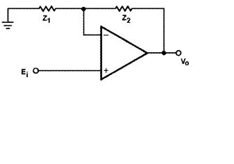
When an electronics engineer has to amplify a given signal, probably his/her first idea is to use a low cost IC operational amplifier (called opamp in the daily electronic jargon). It is linear because the output appears as an enlarged replicated version of the input, with a constant ratio — the gain — between output and input over all the frequency band of interest. Due to practical limitations of these IC's — high but not infinite gain, flat frequency response within specific ranges — (Dostál, 1993), the simple and convenient op-amp needs a few external components (resistors and capacitors) to better define its behavior. In this way, it is possible to implement functions that the op-amp could not perform by itself. Figure 5.1 displays what is probably the simplest arrangement, where Z1 and Z2 are two known impedances.

If the Z's are replaced by ohmic resistors R1 and R2, respectively, applying the two basic rules of the ideal operational amplifiers (i.e., the two input terminals are at the same potential while no current flows into those terminals), Ohm’s law leads to the output/input relationship, or gain,

Vo Ei = −(R2 R1 )

(5.1a)

amply referred to and used in the current literature, technical notes and manuals.

This configuration is handy because simultaneously it allows amplification and sign inversion; thus, it is an inverter. If now the input potential

Figure 5.1. BASIC OPERATIONAL AMPLIFIER: SINGLE INVERTER. It is easily seen that Vo/R2 (or current through R2) is equal to –Ei/R1 (or current through R1) since no current goes into the negative terminal of the amplifier. Besides, the two input terminals (negative and positive) are essentially at zero potential. The two impedances are being taken as ohmic resistors. If, instead, impedance Z1 (or resistor R1) is grounded and the positive terminal connected to an input voltaje Ei, there is no inversión and the gain is given by 1 + R2/R1. The student should work out the demonstration.

302	Understanding the Human Machine

Ei is connected to the positive terminal and R1 is grounded, in other words, if the two input terminals are swapped, the resulting equation becomes,

Vo Ei = (1+ R2 R1 )

(5.1b)

clearly showing that the circuit amplifies without inversion and, for that reason, is usually called non-inverting amplifier. The student is advised to work out the derivation of equation (5.1b) by considering the basic operational amplifier rules. By modifying the external elements in these arrangements (as for example with complex impedances, usually RCnetworks), the range of constant gain can be delimited as a function of the frequency in a selective way.

Are these simple circuits good enough for the detection of biopotentials, fulfilling the basic requirements listed above? The answer is “no”. Its main limitation resides in the common terminal employed for both, the input and the output signals. Besides, such common terminal is also shared with the power supply of the op-amp. In practice, very often neither of the input terminals coincide with the common point and, thus, they cannot be connected to the latter. Most resistance sensor bridges and some kind of transducer configurations illustrate such situation. As a consequence, an amplifier with two floating terminals is required, amplifying the voltage difference between the two. This is precisely a differential amplifier. An instrumentation amplifier, or amplifier for biopotentials, is a precision differential voltage gain device optimized to operate in a noisy environment.

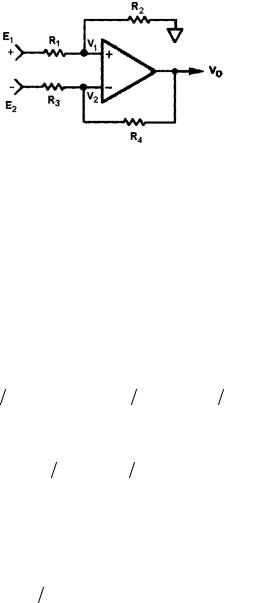
5.3.1. Differential Amplifiers Based on a Single Op-Amp

Figure 5.2 shows a typical and simple configuration to implement a balanced differential amplifier based on a single op amp. Assuming the operational amplifier is ideal (V1 = V2), the output voltage Vo can be calculated by the superposition theorem (Skilling, 1965). The output for E1, when E2 is grounded, is given by,

Vo1 = E1[R2	(R1 + R2 )]×[(R3 + R4 ) R3 ]	(5.2)
where two	factors are included: [(R3 + R4 ) R3 ], the gain of the	non-
inverting amplifier, and the voltage dividing effect of the (R1 , R2 )		net-

work.

Chapter 5. Biological Amplifier

303

Figure	5.2.	BALANCED DIFFERENTIAL AMPLIFIER. When E2 is grounded,
Vo =	Vo1,	and the voltage divider rule leads to E1/V1 = (R1+R2)/R2 and

Vo1/V2 = (R3 + R4)/R3; from the two latter, equation (5.2) is obtained after solving them for V1 and V2, respectively, and equating them. When the other input terminal is grounded, instead, the arrangement coincides with that of Figure 5.1, and Vo = Vo2 is given by equation (5.1a), which now should be written as equation (5.3) is. See text for more details and final result. The student should work out all the algebraic manipulations.

Conversely, when E1 is grounded, we are left with the first case and its output Vo2 is described by eq. (5.1a), or

Vo2 = −E2 (R4 / R3 )	(5.3)
Superposition of the two latter quickly leads to Vo =Vo1 +Vo2 , or,
Vo = E1[R2 (R1 + R2 )]×[(R3 + R4 ) R3 ]− E2 ×(R4 R3 )	(5.4)

If R2 = R4 , R1 = R3 , and the input difference is defined as Ed = E1 − E2 ,

the output voltage can be written as
Vo = (E1 − E2 )×(R4 R3 )= Ed (R4 R3 )	(5.5)

after proper replacements in eq. (5.4), clearly indicating a proportional relationship between output and input, where the ratio R4 / R3 obviously

stands for the circuit differential gain.

Let us now obtain a general expression of the differential gain, without

imposing resistor	symmetry. We merely have to make
E2 = −E1 = −Ei 2	in equation (5.4) because, precisely, a differential

input is characterized by one half of the signal as positive on one of the terminals and the other half as negative on the other terminal, and both

304	Understanding the Human Machine

portions centered against the reference. Moreover, no common input is assumed. Under this condition, equation (5.4) becomes,

Vo = (Ei 2)×{[R2 (R1 + R2 )]×[(R3 + R4 ) R3 ]+(R4 R3 )}

(5.6)

from which it is easily seen that the differential gain Vo/Ei is quantitatively described by,

Gd = (1 2)×{[R2 (R1 + R2 )]×[(R3 + R4 ) R3 ]+(R4 R3 )}

(5.7)

Both eqs. (5.5) and (5.7) coincide when the symmetry condition is imposed on the latter. Besides, they are straightforward and nice (yes, when beauty is found in a mathematical derivation, it means we are understanding and beginning to like the subject).

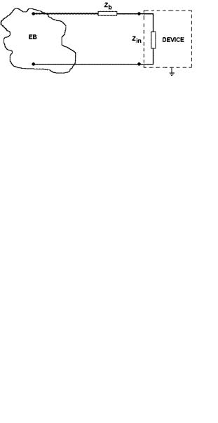
5.3.1.1. Amplifier loading effect

However, there are some restrictions to consider. One of them relates to the amplifier input impedance presented to the biological system. It may become critical when electrodes are directly applied, as in electrocardiography, requiring the concept of impedance matching, or adaptation, in order to guarantee efficient signal transference. Keeping always in mind the ideal op-amp (Figure 5.2), the input impedances for E1 and for E2 ,

respectively, are (R1 + R2 ) and R3 (remember the potential V2 is a virtual zero); in fact, since V1 is nearly equal to V2 , the former could be reduced to only R1 . Thus, when looking from the biological system, the amplifier’s input impedance is given by (R1 + R3 ), which combined with

the output impedance of the biological source, acts as voltage divider so decreasing the actual input signal (Figure 5.3). In other words, the latter loads the original voltage.

Thus, it is important to make the amplifier input impedance significantly

Figure 5.3. LOADING EFFECT OF THE INPUT IMPEDANCE OF THE AMPLIFIER.

Chapter 5. Biological Amplifier	305
higher than the output impedance of	the biological element, that is,

Zin >> Zb ; the higher, the better. Since gains much larger than 10 are desirable, due to the high input impedance requirement, R2 and R4

should take high values. However, values greater than 10 MΩ are not recommendable because susceptibility to noise also goes up. Their tolerance is usually large (about 20 %) and their quality tends to be poorer. On the other hand, if one lowers tolerance to improve circuit performance, the whole configuration becomes more expensive. Hence, a compromise should be reached.

Suggested exercise: Design a symmetric amplifier according to the diagram of Figure 5.2 connected to a biological system with a 500 Ω output impedance. The required gain is 50 and the actual signal between E1 and E2 should not be lower than 0.95 the original source signal Eb. Resistors larger than 200 KΩ are not recommended. Redesign the resistors if the actual signal were to be 0.9 and 0.99 of Eb, respectively. Discuss the practical limitations, if any, in all three cases.

5.3.1.2. External resistors mismatch

Another limitation of this arrangement rests on the intrinsic practical mismatch of all four external resistors (ratios should be kept, aiming at the best possible circuit symmetry, which means the so called resistor’s pairing or matching); otherwise, an imbalanced output is produced (Pallàs–Areny & Webster, 1999). Let us define the common mode input voltage Ec as

Ec = (E1 + E2 ) 2

(5.8)

which is reflected at the output multiplied by the common mode gain Gc , while the differential input voltage Ed appears multiplied by the

differential gain Gd , so that the total output, by superposition, is in fact,

Vo = Gc Ec + Gd Ed

(5.9)

However, by definition of differential amplifier, the common mode gain should be zero or at least tend to zero, getting again a relationship as shown in equation (5.5). In practice, Gc has a finite value different from

zero and can be experimentally obtained as the quotient between the output voltage Vocm and the input voltage, when the same value E1 = E2 = Ei

306	Understanding the Human Machine

with respect to the reference is applied to both terminals. Thus, by making use of equation (5.4), we get

Vocm = Ei ×{[R2 (R1 + R2 )]×[(R3 + R4 ) R3 ]−(R4 R3 )}	(5.10)
which, after dividing through by Ei , leads into
Gc =[R2 (R1 + R2 )]×[(R3 + R4 ) R3 ]−(R4 R3 )	(5.11)

as a full expression of the common mode gain.

Suggested exercise: Say that the four resistors in Figure 5.2 are equal (R1 = R3 = R4 = R), but one of them, R2, is 0.1 % off its nominal value, that is, it is either 0.99xR or 1.01xR, depending on whether it deviates in excess or defect. Replacing these values in eq. (5.11) yields a common gain Gc = –0.00503 and 0.00498, respectively, obviously small, finite and different from zero. Repeat the exercise when the deviation is 0.01, 1 and 5%. Discuss.

5.3.1.3. Common Mode Rejection (CMR)

Since in real life we have to deal with imperfect technological elements, this amplifier always handles the two gains introduced above, one large and the other small. Hence, it appears convenient to define a combined parameter in order to quantify how high the differential gain and how low the common mode gain are. Such parameter, extremely important in the biological amplifier, is the Common Mode Rejection Ratio (CMRR), or

CMRR = Gd Gc

(5.12a)

simply defined as the ratio of the two gains. Another definition also in use is as the logarithm of the ratio, or

CMRR[dB]= 20×log(Gd Gc )

(5.12b)

obviously measured in decibels. Conceptually, it does not add anything; it is just an alternative. Both equations (5.12) must be emphasized because of their paramount importance in this kind of amplifier.

In the numerical example given above, since the differential gain is 1 ( Gd = R4 R3 , with both resistors equal to R), and rounding up an abso-

lute common gain of 0.005, we end up with a CMR = 46 dB. In most of their applications, instrumentation amplifiers require CMR’s > 80 dB, while in cases where a resistive transducer bridge is involved, 120 dB or even more may be needed. The example shows that an increase of the differential gain to 10, with the same single resistance offset of only 0.1

Chapter 5. Biological Amplifier

307

%, raises the CMR to 66 dB without reaching yet the necessary levels. The student is invited to try different numbers in order to get a feeling of the restrictions and possible practical difficulties.

Pairing of the external elements is a desirable condition and definitely should be sought. Maximum pairing is reached when Gc in equation

(5.11) is forced to be zero, or,
[R2 (R1 + R2 )]×[(R3 + R4 ) R3 ]−(R4 R3 )= 0	(5.13)
easily leading to,
R4 R3 = R2 R1	(5.14)

as the practical condition to be met, better explaining the reason to search for symmetry. Nonthe less, usually it is not easy to obtain, thereby limiting the actual common mode rejection. Besides, as already mentioned, its input impedance is also limited. For these reasons, the single op-amp configuration is rarely used, if ever.

5.3.2. Differential Amplifiers Based on Two Op-Amps

The two-amplifier approach shown in Figure 5.4 is basically formed by

Figure 5.4. TWO OP-AMP BIOLOGICAL AMPLIFIER.