Cohen M.F., Wallace J.R. - Radiosity and realistic image synthesis (1995)(en)

CHAPTER 6. RENDERING

6.2 MESH CHARACTERISTICS AND ACCURACY

Figure 6.15: Conforming versus nonconforming elements.

along boundaries, thus ensuring C0 continuity at the boundaries. In practice, this means that T-vertices (defined in Figure 6.15) must be avoided. Conformance is not an issue for constant elements, which are often used during the radiosity solution, but it is critical for rendering, where linear or higher-order elements are normally used.

6.2.5 Discontinuities

If light sources have a constant emission value (or are C∞ ) across the surface and if changes in visibility are ignored, then the radiosity function B(x) across a receiving surface will be continuous in all derivatives (i.e., it will also be C∞ ). This is evident from the form factor kernel, G(x, x′), which itself is C∞ except where the visibility term V(x, x′) changes from one to zero, and at singularities where x and x′ meet and the denominator goes to 0.

If changes in visibility (i.e., shadows) are included, the radiosity function can contain discontinuities of any order [121]. Discontinuities in value and in the first and second derivatives are the most important, since these often provide visual cues to three-dimensional shape, proximity, and other geometric relationships. Much of the “image processing” performed by the eye involves enhancing such discontinuities and, as a result, the failure to reproduce discontinuities correctly can degrade image quality dramatically.

Radiosity and Realistic Image Synthesis	149
Edited by Michael F. Cohen and John R. Wallace

CHAPTER 6. RENDERING

6.2 MESH CHARACTERISTICS AND ACCURACY

Figure 6.16: Shadows can cause 0th, 1st, 2nd, and higher-order discontinuities in the radiosity function across a surface.

Value Discontinuities

Discontinuities in the value of the radiosity function occur where one surface touches another, as at letter a of Figure 6.16. In Figure 6.17 the actual radiosity function is discontinuous in value where the wall passes below the table top. The shading should thus change abruptly from light to dark at the boundary defined by the intersection of the wall and the table. Unfortunately, the boundary falls across the interior of elements on the wall. Instead of resolving the discontinuity, interpolation creates a smooth transition and the shadow on the wall appears to leak upwards from below the table top.

Incorrectly resolved value discontinuities can also cause “light leaks,” in which interpolation across one or more discontinuities causes light to appear where shadow is expected. In Figure 6.18, for example, elements on the floor pass beneath the wall dividing the room. The resulting light leak gives the incorrect impression of a gap between the wall and the floor. The problem is compounded when these elements incorrectly contribute illumination to the room on the left, which is totally cut off from the room containing the light source.

Derivative Discontinuities

Discontinuities in the first or second derivative occur at penumbra and umbra boundaries (letter b of Figure 6.16), as well as within the penumbra. When mesh elements span these discontinuities, interpolation often produces an inaccurate and irregular shadow boundary. The staircase shadows in Figure 6.2 are an example.

Radiosity and Realistic Image Synthesis	150
Edited by Michael F. Cohen and John R. Wallace

CHAPTER 6. RENDERING

6.2 MESH CHARACTERISTICS AND ACCURACY

Figure 6.17: Failure to resolve a discontinuity in value. This is a closeup of the radiosity solution shown in Figure 6.2.

Figure 6.18: A light leak caused by failure to resolve discontinuities in value where the dividing wall touches the floor. The dividing wall completely separates the left side of the room from the right side, which contains the light source.

Radiosity and Realistic Image Synthesis	151
Edited by Michael F. Cohen and John R. Wallace

CHAPTER 6. RENDERING

6.2 MESH CHARACTERISTICS AND ACCURACY

Singularities in the first derivative can also occur, as at letter c of Figure 6.16 where the penumbra collapses to a single point. Tracing along the line of intersection between the two objects, an instantaneous transition from light to dark is encountered at the corner point. The first derivative is infinite at that point, although the function is continuous away from the boundary.

The correct resolution of discontinuities requires that they fall along element boundaries, since the approximation is always C∞ on element interiors. Thus, discontinuity boundaries must either be determined before meshing or the mesh must adapt dynamically to place element edges along the discontinuities. Since discontinuities may be of various orders, interpolation schemes that can enforce the appropriate degree of continuity at a particular element boundary are also required. Techniques for finding and reconstructing discontinuities will be discussed in detail in Chapter 8.

Continuity at Geometric Boundaries

Discontinuities in value occur naturally at boundaries where the surface normal is discontinuous, such as where the edge of the floor meets a wall. Such discontinuities are normally resolved automatically, since surfaces are meshed independently.

A problem can occur, however, if the boundaries of the primitives generated by a geometric modeler do not correspond to discontinuities in the surface normal. For example, curved surfaces will often be represented by collections of independent polygonal facets. If the facets are meshed independently, adjacent elements will often be nonconforming across facet boundaries, and shading discontinuities will result, as shown in Figure 6.19. It is easiest to maintain conformance in this case if the connectivity of the facets is determined prior to meshing and the surface is meshed as a single unlit (see Figure 6.20). This approach is used by Baum et al. [18] for the special case of coplanar facets. Better yet, the radiosity implementation should allow the user to enter the faceted surfaces as a topologically connected primitive such as a polyhedron.

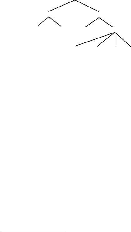
6.3 Automatic Meshing Algorithms

With a better understanding of how various mesh attributes affect the accuracy of the solution, it is now possible to discuss automatic meshing strategies. A taxonomy of automatic meshing algorithms is shown in Figure 6.21.3

3Although user intervention can be helpful in constructing a mesh, the discussion in this chapter will be limited to automatic mesh generation. Meshes for engineering applications are still often constructed with some interactive help, but good results require an experienced user who understands the underlying principles of the analysis. In image

Radiosity and Realistic Image Synthesis	152
Edited by Michael F. Cohen and John R. Wallace

CHAPTER 6. RENDERING

6.3 AUTOMATIC MESHING ALGORITHMS

Figure 6.19: The polygonal facets representing the curved surface in this image were meshed independently. The resulting elements are nonconforming at the facet boundaries, causing shading discontinuities.

Figure 6.20: The facets in this image were connected topologically prior to meshing, and the surface was meshed as a unit.

Radiosity and Realistic Image Synthesis	153
Edited by Michael F. Cohen and John R. Wallace

CHAPTER 6. RENDERING

6.3 AUTOMATIC MESHING ALGORITHMS

	Automatic Meshing Strategies
No Knowledge of Function		Knowledge of Function
Uniform	Non-Uniform	A Priori	A Posteriori

r-refinement h-refinement p-refinement remeshing

Figure 6.21: A taxonomy of automatic meshing strategies.

Meshing algorithms can be broadly classified according to whether or not they use information about the behavior of the function to be approximated. Although obtaining an optimal mesh normally requires such knowledge, in practice some degree of meshing without it is almost always necessary. Meshing in this case generally means subdividing as uniformly as possible (although subdividing complex geometries may require a nonuniform mesh). Algorithms for producing a uniform mesh are described in Chapter 8.

Meshing techniques that use knowledge of the function can be characterized as either a priori or a posteriori [211]. A priori methods specify all or part of the mesh before the solution is performed. Discontinuity meshing, in which discontinuity boundaries associated with occlusion are determined prior to the solution based on purely geometric considerations, is an a priori method. A priori algorithms, including discontinuity meshing, are discussed in Chapter 8.

A posteriori algorithms determine or refine the mesh after the solution has been at least partially completed. An initial approximation is obtained using a uniform or other mesh determined a priori. The mesh is then refined in regions where the local error is high, using information provided by the initial approximation of the function, such as the gradient, to guide decisions about element size, shape, and orientation. A posteriori meshing strategies are the subject of the remainder of this chapter.

6.3.1 A Posteriori Meshing

A posteriori meshing algorithms common to finite element analysis can be categorized as follows [211]:

synthesis the analysis of illumination is typically not the user’s primary task, and the detailed specification of a mesh is intrusive and often beyond the user’s expertise.

Radiosity and Realistic Image Synthesis	154
Edited by Michael F. Cohen and John R. Wallace

CHAPTER 6. RENDERING

6.3AUTOMATIC MESHING ALGORITHMS

•r-refinement : reposition nodes

•h-refinement : subdivide existing elements

•p-refinement : increase polynomial order of existing elements

•remeshing: replace existing mesh with new mesh

Each of these approaches addresses one or more of the basic mesh characteristics discussed earlier: mesh density, basis function order, and element shape. Radiosity algorithms have so far relied almost exclusively on h-refinement. However, the other approaches will also be briefly described here, partly to indicate possible directions for radiosity research. See Figure 6.22 for illustrations of these approaches.

R-refinement

In r-refinement the nodes of the initial mesh are moved or relocated during multiple passes of mesh relaxation. At each pass, each node of the mesh is moved in a direction that tends to equalize the error of the elements that share the node. (See section 8.4 for a basic algorithmic approach to moving the vertices.) The function is then reevaluated at the new node locations. Relaxation can continue until the error is evenly distributed among the elements.

R-refinement has the advantage that the mesh topology is not altered by the refinement, which may simplify algorithms. It generates an efficient mesh, in that it minimizes the approximation error for a given number of elements and nodes. On the other hand, r-refinement cannot guarantee that a given error tolerance will be achieved. Since the number of elements is fixed, once the error is evenly distributed it can’t be lowered further. Also, care must be taken during relocation not to move nodes across element boundaries. It may furthermore be difficult to maintain good element shape near fixed boundaries.

H-refinement

In h-refinement, the local error is decreased by increasing the density of the mesh; elements with a high error are subdivided into smaller elements. (The “h” refers to the symbol commonly used to characterize element size in finite element analysis.) The function is then evaluated at the new nodes. Since new nodes are added, the approximation error can be made as small as desired (although this may not always be practical). Elements and nodes can also be removed in regions where the approximation error is lower than necessary. In some h-refinement algorithms, refinement does not require reevaluation of the function at existing nodes.

Radiosity and Realistic Image Synthesis	155
Edited by Michael F. Cohen and John R. Wallace

CHAPTER 6. RENDERING

6.3 AUTOMATIC MESHING ALGORITHMS

Figure 6.22: Basic a posteriori meshing strategies.

However, the inability to move existing nodes restricts the ability of h- refinement to reduce error by adjusting element shape or orientation. As a result, h-refinement can be inefficient, in that more elements than necessary may be needed to reach a desired accuracy. Special handling is required to maintain continuity between elements subdivided to different levels of refinement. H-refinement algorithms must also pay careful attention to mesh grading. Radiosity implementations have relied almost exclusively on a variety of h- refinement algorithms. These are expanded on in section 6.3.2. Babuska et al. [15] provide a valuable source for h-refinement and p-refinement approaches used in engineering applications.

Radiosity and Realistic Image Synthesis	156
Edited by Michael F. Cohen and John R. Wallace

CHAPTER 6. RENDERING

6.3 AUTOMATIC MESHING ALGORITHMS

P-refinement

In p-refinement, the approximation error is reduced by increasing the order of the basis functions for certain elements. (The symbol “p” refers to the polynomial order of the basis functions.) New nodes are added to the affected elements, but the element shape and the mesh topology are not otherwise changed. In contrast to h-refinement, the number of elements in the mesh is not increased, which limits computational costs in some ways. However, the function must be evaluated at additional nodes, and the higher-order basis functions can be more expensive to compute. As with h-refinement, the ability to change element shape or orientation is restricted. Care must also be taken to maintain continuity between adjacent elements having basis functions of different orders.

Remeshing

Remeshing algorithms modify both the node locations and mesh topology; in essence the existing mesh is completely replaced. This allows complete flexibility of element shape and orientation, as well as the ability to decrease arbitrarily the approximation error. Following remeshing, the function must be reevaluated at the nodes of the new mesh.

Hybrid Methods

Hybrid refinement methods can be constructed by combining the above basic approaches. For example, r-refinement works best when it begins with a mesh that is reasonably well refined, since relaxation cannot reduce the local error beyond the minimum achievable with the initial number of nodes. A potentially useful hybrid strategy might thus use h-refinement to achieve a reasonable initial sampling density and r-refinement to more evenly distribute the approximation error.

6.3.2 Adaptive Subdivision: H-refinement for Radiosity

Almost all a posteriori meshing algorithms for radiosity have used h-refinement. This approach, commonly called adaptive subdivision in radiosity applications, follows the basic outline of an a posteriori method: a solution is computed on a uniform initial mesh, and the mesh is then refined by subdividing elements that exceed some error tolerance.

Figure 6.23 illustrates the improvement provided by adaptive subdivision over the uniform mesh approximation shown at the beginning of the chapter in Figure 6.2. The image quality is improved compared to that provided by the high uniform mesh resolution of Figure 6.6, while using the same number of

Radiosity and Realistic Image Synthesis	157
Edited by Michael F. Cohen and John R. Wallace

CHAPTER 6. RENDERING

6.3 AUTOMATIC MESHING ALGORITHMS

Figure 6.23: Adaptive subdivision. Compare to Figure 6.2.

Figure 6.24: Error image for adaptive subdivision. Compare to Figures 6.4 and 6. 7.

Radiosity and Realistic Image Synthesis	158
Edited by Michael F. Cohen and John R. Wallace