Cohen M.F., Wallace J.R. - Radiosity and realistic image synthesis (1995)(en)

CHAPTER 4. THE FORM FACTOR

4.9. EVALUATING THE INNER INTEGRAL

Figure 4.16: Malley’s method.

4.9.5 Monte Carlo Ray Tracing

Ray tracing (as opposed to scan conversion and the Z-buffer) provides an extremely flexible basis for evaluating the visibility term in the numerical integration of the form factor equation. Because rays are cast independently they can be shot to and from any distribution of points on the elements or directions in the hemisphere. Nonuniform and adaptive sampling can be used to distribute computational effort evenly. Rays can also be distributed stochastically, which can render the effects of inadequate sampling less noticeable by converting aliasing to noise.

In addition, ray tracing handles a wide variety of surface types, including curved surfaces, and a number of efficiency schemes to accelerate ray intersections exist. A disadvantage of ray tracing is that the expense per quadrature point will generally be higher since coherency from ray to ray is more difficult to exploit than in scan conversion algorithms.

Ray casting provides an excellent basis for Monte Carlo integration of the form factor equation over the hemisphere. In equation 4.9, the kernel contains the factor cos θi . Thus importance sampling can be performed by selecting directions over the hemisphere with a sample density proportional to the cosine. In this way, more effort will be expended where the form factor is largest. Since the density of rays is then proportional to the differential form factor, each sample will carry equal weight.

Malley describes a straightforward method for generating a set of sample

Radiosity and Realistic Image Synthesis	89
Edited by Michael F. Cohen and John R. Wallace

CHAPTER 4. THE FORM FACTOR

4.9. EVALUATING THE INNER INTEGRAL

directions with the desired distribution [157]. Malley’s method is essentially a Monte Carlo evaluation of the Nusselt analog (see Figure 4.8) run in reverse. He begins by generating a set of random points uniformly distributed in the circle10 under the hemisphere (see Figure 4.16).11 To determine a direction to shoot a ray, one of these points is projected vertically to intersect the hemisphere. The ray is then directed radially out from the center of the hemisphere through this projected point. Rays are shot in this manner for every sample point in the circle. The number of times each element in the scene is hit by a ray is recorded. The form factor is then given by the number of rays that hit a given element divided by the total number of rays shot. Referring back to Nusselt’s analog, the total number of rays shot is an estimate of the area of the circle covered by the double projection. The fraction of the total rays that hit a given element thus approximates the area of the projection of the element on the hemisphere base, relative to the total area of the base. This fraction is equal to the form factor. Maxwell also describes the computation of form factors with ray tracing [164].

4.9.6 Area Sampling Algorithms

The hemisphere sampling algorithms described in the previous sections are most efficient when form factors to all elements from a single point must be computed at once. Certain solution techniques (e.g., the progressive radiosity algorithm described in the next chapter) require form factors between only a single pair of elements at a time, thus the full hemisphere methods are inefficient. In this case, the area-area formulation (equation 4.7) is a more efficient basis for algorithm development.

For convenience, the equation for the form factor from a differential area i to a finite element j is repeated

FdAi → Aj = òAj	cos θi cos θ j	Vij dAj .	(4.27)
	π r2

The integration can be performed by evaluating the kernel at randomly distributed points for a Monte Carlo solution. Wang’s discussion of Monte Carlo sampling of spherical and triangular luminaires in [248] contains much practical information that can be applied to form factor integration.

10A random set of points in a circle can be derived by generating two random numbers between 0 and 1 to locate a point in the square surrounding the circle. If the point is in the circle, use it; if not discard it. Independently generating a random angle and radius will not result in a uniform distribution of points.

11These points are only used to determine a direction, not to select a point to start a ray. For an area-to-area computation, the ray origin can also be stochastically distributed over the area of the element.

Radiosity and Realistic Image Synthesis	90
Edited by Michael F. Cohen and John R. Wallace

CHAPTER 4. THE FORM FACTOR

4.9. EVALUATING THE INNER INTEGRAL

Figure 4.17: Numerical integration of form factor from differential area to finite area.

Alternatively, the integration can be performed by subdividing the area uniformly. Wallace et al. subdivide Aj into a set of m smaller areas Ajk and select a sample point at the center of each subarea (see Figure 4.17). The form factor then becomes

m	cos θ k	cos θ k
FdAi — A j = å	i				j	V(dAi , Ajk ) Ajk	(4.28)
	π(r	k	)	2
k=1

The equation is evaluated by shooting a ray from dAi to each delta area to

determine the visibility, V(dAi ,	Ajk ). The contributions	of those delta	areas
that are visible is then summed.
Equation 4.28 assumes that the subareas are reasonable approximations to
differential areas, which is the	case only if Ajk <<	r2. Otherwise,	Ajk

should be treated as a finite area. For example, each term of the summation could evaluate the exact polygon form factor formula for the particular subarea, as discussed in Tampieri in [230].

A less expensive alternative is to approximate Ajk by a finite disk of the same area, as suggested by Wallace et al. [247]. The analytic formula for a point- to-disk form factor can then be substituted into the summation of Equation 4.28.

The form factor from a differential area to a directly opposing disk of area	Aj
Radiosity and Realistic Image Synthesis	91
Edited by Michael F. Cohen and John R. Wallace

CHAPTER 4. THE FORM FACTOR

4.9. EVALUATING THE INNER INTEGRAL

Figure 4.18: Configuration for approximation of the form factor from a differential area to arbitrarily oriented disk.

is

FdAi → Aj =	Aj		(4.29)
	π r2 + A
		j

The effect of element orientation can be approximated by including the cosines of the angle between the normal at each surface and the direction between the source and the receiver (see Figure 4.18):

FdAi → Aj =	Aj cos θi	cos θ j		(4.30)
	π r2 +	A	j

The form factor from a differential area to an element j approximated by a set of m disks of area Aj /m is thus

m	cos θ k			cos θ k
FdAi → A j = Aj å		i				j	V(dAi , Aj )	(4.31)
	π (r	k	2		A j
k =1		)		+
					m

The reciprocity relationship can also be used to approximate the form factor from a finite area to a differential area through the ratio of the areas:

FAj → dAi = FAj → dAi	dA		=	cos θi	cos θ j			(1.32)
		i					dAi
	A	j		π r2	+ A	j

The disk approximation breaks down when the distance from the disk to the receiver is small relative to the size of the delta area, and visible artifacts may result, as shown in Figure 4.19(a). An additional difficulty with uniform subdivision of the element is that since a single ray is cast to each of the source subdivisions, the element is essentially treated as several point lights as far

Radiosity and Realistic Image Synthesis	92
Edited by Michael F. Cohen and John R. Wallace

CHAPTER 4. THE FORM FACTOR

4.9. EVALUATING THE INNER INTEGRAL

Figure 4.19: (a) Artifacts introduced by the disk approximation. The receiving surface consists of 30 by 30 elements. (b) Adaptive subdivision of the source element for a typical node on the receiving element.

as visibility is concerned. As a result, the shadow boundary may appear as a number of overlapping, sharp-edged shadows rather than a smoothly shaded penumbra.

Both of these problems can be addressed by adaptively subdividing area Aj . This is performed in a straightforward manner by subdividing the area recursively until the resulting delta areas fulfill some criterion. The criterion may be geometric (e.g., the delta area must be much less than r2) or based on the energy received from the delta area. The result of adaptive element

Radiosity and Realistic Image Synthesis	93
Edited by Michael F. Cohen and John R. Wallace

CHAPTER 4. THE FORM FACTOR

4.10 FULL AREA-TO-AREA QUADRATURE

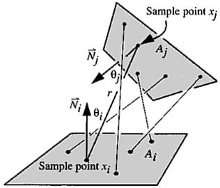
Figure 4.20: Monte Carlo area-to-area form factor.

subdivision is shown in Figure 4.19(b). Tampieri [230] provides a detailed practical discussion of this approach, including pseudocode.

4.10 Full Area-to-Area Quadrature

Any of the analytic or numeric differential area-to-area form factor solutions discussed so far can be used to approximate the full area to area form factor. The differential area-to-area form factor is evaluated at one or more points on element Ai and the result averaged. For example, the ray tracing algorithm just described could be performed for several points on Ai . However, since many rays connecting the two surfaces originate at the same points on Ai , this approach samples Ai inefficiently. There are several more effective approaches, including Monte Carlo integration, numerical solution of the contour integral form, and hierarchical subdivision.

4.10.1 Monte Carlo Integration

The double area integral can be approximated more accurately by distributing the endpoints of the rays over Ai as well as Aj. In a Monte Carlo approach ray endpoints on both elements would be distributed randomly, or according to some quasi-random distribution like the Poisson disk. Pseudocode is for a

Radiosity and Realistic Image Synthesis	94
Edited by Michael F. Cohen and John R. Wallace

CHAPTER 4. THE FORM FACTOR

4.11. CONTOUR INTEGRAL FORMULATION

simple area-to-area Monte Carlo form factor algorithm is given in Figure 4.21
(the geometry is shown in Figure 4.20).
Fij = 0
for k = 1 to n
randomly select point xi				on element i		or use stratified sample
randomly select point xj				on element j		or use stratified sample
determine visibility between xi and xj
if visible
compute r2 = (x		i	–x	)2
			j
compute cosθj	= rij			•	Ni
compute cosθj	= rij			•	Nj
compute F = cosθicosθ j
			pr2 + Aj
					n
if( F > 0 ) Fij = Fij				+	F
end if
end for
Fij = Fij * Aj

where rij is the normalized vector from xi to xj, and N i is the unit normal to element i at point xi (and vice versa for switching i and j).

Figure 4.21: Pseudocode for Monte Carlo area-to-area form factor computation.

One can do better in terms of fewer rays by sampling the elements nonuniformly and adaptively. An elegant solution for this decision-making process is presented in Chapter 7.

4.11 Contour Integral Formulation

In the earliest work introducing the radiosity method to computer graphics, Goral et al. [100] used Stokes, theorem to convert the double area integral into the double contour integral of equation 4.10.

The contour integrals can be evaluated numerically by “walking,, around the contours of the pair of elements,12 evaluating the kernel at discrete points and summing the values of the kernel at those points [100]. In fact, Goral et al. use a three-point quadratic Gaussian quadrature (nine-point in 2D) along

12Nishita and Nakamae point out that the contour integration approach can be used to compute a single form factor to objects constructed of multiple non-coplanar surfaces. The form factor computed for the contour of the composite object as viewed from the differential area is equal to the sum of the form factors to each of the component surfaces, since it is the solid angle subtended by the surfaces of the object that determines their contribution to the form factor. This is a valuable observation that has not yet been taken advantage of in radiosity implementations for image synthesis.

Radiosity and Realistic Image Synthesis	95
Edited by Michael F. Cohen and John R. Wallace

CHAPTER 4. THE FORM FACTOR

4.12 A SIMPLE TEST ENVIRONMENT

Figure 4.22: Simple test environment.

the boundaries. Care must be taken when the boundaries are shared between elements, as ln(r) is undefined as r → 0.

Equation 4.10 does not account for occlusion. It only the inner contour integral is to be evaluated (in computing, a differential area-to-area form factor), occlusion can be accounted for using a polygon clipping approach such as Nishita and Nakamae’ s [175].

4.12 A Simple Test Environment

To provide a concrete illustration of some of the issues discussed in this chapter, three numerical form factor algorithms have been tested on the simple twopolygon environment shown in Figure 4.22. Results are shown in Figure 4.23. The two polygons are parallel unit squares one unit distance apart. The analytic form factor between them is approximately 0.1998.

Tests were run using the hemicube method, Malley’s method for randomly selecting directions, and the area-area Monte Carlo method. In each case, two tests were run, (Test 1) from the center point only of element i, and (Test 2) from a set of randomly selected points in element i. A series of 1000 runs was made of each. The mean, standard deviation (box height in graph) and minimum and maximum values (vertical lines) are displayed in the graphs.13 The horizontal axis is given in terms of the resolution of the hemicube, the number of random directions that fell in element j in Malley’s method and the number of sample points in element j in the Monte Carlo method. In Test 2, the same number

13The hemicube method from the center of element i (Test 1) has no deviation since it is a deterministic algorithm.

Radiosity and Realistic Image Synthesis	96
Edited by Michael F. Cohen and John R. Wallace

CHAPTER 4. THE FORM FACTOR

4.12 A SIMPLE TEST ENVIRONMENT

Figure 4.23: Test results on parallel elements. In Test1, only the center point was chosen on element i and n points on element j. In Test 2 n points are chosen on both elements. res is the resolution of the hemicube in both tests.

Radiosity and Realistic Image Synthesis	97
Edited by Michael F. Cohen and John R. Wallace

CHAPTER 4. THE FORM FACTOR

4.13. NONCONSTANT BASIS FUNCTIONS

was chosen for sample points in element i and the horizontal axis represents the product of the number of sample points and directions.

All of the methods converged reasonably well in this case as the sampling density (resolution, in the case of the hemicube) increased. Note that the form factor from the center of element i to element j is approximately 0.2395, and thus the solution always converged to about 20% over the actual value for Test 1. Also, note the single point on the graph for the hemicube with resolution 2 performed at 2 random points chosen on element i. Because of the low resolution and the fixed orientation of the hemicube with respect to the environment coordinate frame, the form factor happens always to be the same, no matter where the hemicube is position on element i. This extreme case highlights the problems due to the regular sampling enforced by the hemicube that are encountered as the resolution becomes small relative to the projected area of the elements.

4.13 Nonconstant Basis Functions

The discussion so far has been limited to evaluating form factors where constant basis functions are used. This has been the dominant approximation used in radiosity implementations to date. In this section we briefly introduce the computation of form factors for higher order elements. However, this remains largely an area for future development.

Recall from the last chapter that the coefficients of the linear operator K are given by

Kij = Mij –ρiFij

(4.33)

For orthonormal (e.g., constant) bases the M matrix is simply the identity after division by “area” terms. In the more general case, it represents the inner product of the ith and jth basis functions:

Mij = òs Ni(x) Nj(x) dA

(4.34)

The integral will be nonzero only where the support of the two basis functions overlaps. This integral can generally be evaluated analytically since the basis functions are chosen to be simple polynomials.

Slightly reorganizing equation 4.3, the Fij are given by

Fij = òAi òA j Ni (x) N j (x9) G(x, x9) dA9 dA

(4.35)

The interpretation of the coefficients Fij is slightly less intuitive in this general case. The integral is still over the support (Ai, Aj) of the two basis functions

Radiosity and Realistic Image Synthesis	98
Edited by Michael F. Cohen and John R. Wallace