Cohen M.F., Wallace J.R. - Radiosity and realistic image synthesis (1995)(en)

CHAPTER 4. THE FORM FACTOR

4.9. EVALUATING THE INNER INTEGRAL

This type of importance sampling will be used, for example, to distribute samples according to the cosine in the form factor integral to reduce the number of expensive visibility evaluations. Explicit inverses for P(x) may be difficult to derive, in which case analog procedures, or precomputed lookup tables may be useful. Malley’s method, discussed in section 4.9.5, is an example of this approach.

Monte Carlo integration in general is a broad topic, to which numerous textbooks and articles are devoted. Monte Carlo integration for image synthesis is discussed in greater detail in [71, 135, 147, 215]

4.9 Evaluating the Inner Integral

The area-area and the area-hemisphere forms of the double integral both share the same outer integral over element i. Thus, one can separate the question of evaluating the full integral into two parts: first, the evaluation of the inner integral from some dAi , and second, the selection of one or more sample points on element i at which to evaluate the inner integral. If points on element i are chosen with an even distribution then the full integral is the average of the inner integral evaluations.

In fact, many implementations use only one representative point on element i, in essence making the following assumption (valid also for the area-area form):

Fij =	1	òAi òΩ Giω dω dAi ≈ òΩ Giω dω at sample point xi	(4.22)
	Ai

This assumes that the inner integral is constant across element i, which may be reasonable when the distance (squared) is much greater than the area of element j. However, changes in visibility between elements i and j also affect the validity of this approximation. Whether or not this assumption is used, or the inner integral is evaluated at many sample points in element i, one is left with the problem of evaluating the inner integral. This will be the topic of the following sections.

4.9.1 Hemisphere Sampling Algorithms

The use of the hemispherical integral provides a direct basis for evaluating the form factor from a differential area, dAi , to all elements simultaneously. The geometric kernel, Giω , is given by

G =	cos θi	V		(4.23)
iω	π		ij
Radiosity and Realistic Image Synthesis				79
Edited by Michael F. Cohen and John R. Wallace

CHAPTER 4. THE FORM FACTOR

4.9. EVALUATING THE INNER INTEGRAL

The visibility term, Vij , which is 1 if element j is visible in direction d ω , is the computationally expensive part of the kernel evaluation. Determining the visibility of an element j in a particular direction involves intersecting a ray emanating from dAi with element j and with all surfaces that may block the ray.

Since form factors from element i to all elements are needed eventually, there is a clear advantage in performing the visibility calculation once and simply summing a differential form factor into Fik , where element k is the element “seen” in direction d ω from dAi. Thus, a single integration over the hemisphere results in a full row of differential area-to-element form factors. Given this observation, the question is how to sample the hemisphere of directions above dAi , and how to perform the visibility calculations in the chosen directions.

Hemisphere sampling approaches can be principally differentiated by the hidden surface algorithm they use. Certain algorithms provide efficiency by exploiting coherence in the geometry of visible surfaces, while others provide flexibility for stochastic, adaptive or nonuniform sampling. A geometric analog to the differential area-to-area form factor equation is given first to provide some useful intuition for the algorithms that follow.

4.9.2 Nusselt Analog

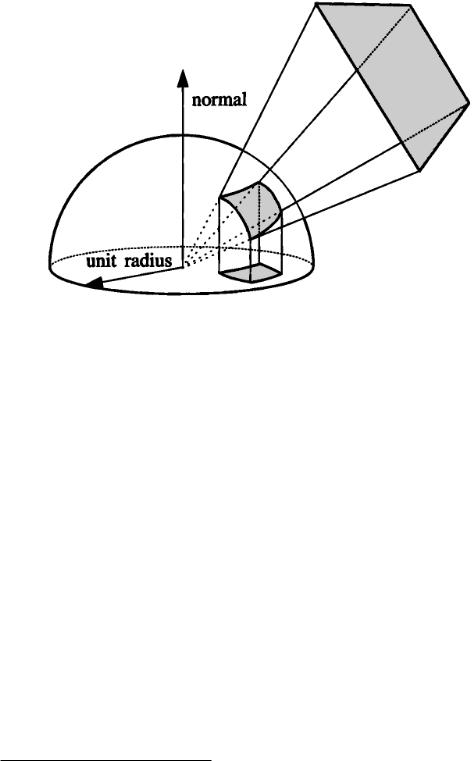
The Nusselt analog provides a geometric analog to the differential area-to-area form factor equation 4.7 (ignoring the visibility factor). An imaginary unit hemisphere is centered on the differential area, as in Figure 4.8. The element is projected radially onto the hemisphere and then orthogonally down from the hemisphere onto its base. The fraction of the base area covered by this projection is equal to the form factor.

Why does this work? The area of the projection of the element on the unit hemisphere is equal to the solid angle subtended by the element, by definition of the solid angle, and thus accounts for the factor cos θj /r2. The projection down onto the base accounts for the cos θi term, and the π in the denominator is the area of a unit circle.

In heat transfer applications, form factors have sometimes been computed for complex shapes by evaluating the Nusselt analog photographically, using a fisheye lens that effectively performs the same double projection. The area covered by the object in the resulting photograph is measured manually to obtain the form factor.

4.9.3 The Hemicube

The Nusselt analog illustrates the fact that elements covering the same projected area on the hemisphere will have the same form factor, since they occupy the

Radiosity and Realistic Image Synthesis	80
Edited by Michael F. Cohen and John R. Wallace

CHAPTER 4. THE FORM FACTOR

4.9. EVALUATING THE INNER INTEGRAL

Figure 4.8: Nusselt analog. The form factor from the differential area dAi to element Aj is proportional to the area of the double projection onto the base of the hemisphere.

same solid angle. Likewise, if an element is projected radially onto any intermediate surface, as in Figure 4.9, the form factor for the projection will be the same as for the element itself. This observation forms the basis for the hemicube form factor algorithm, in which elements are projected onto the planar faces of a half cube instead of onto a hemisphere [62].

A hemicube is placed around a differential area (see Figure 4.10), with the hemicube faces subdivided into small grid cells. Each grid cell defines a direction and a solid angle. A delta form factor, F, is computed for each cell based on its size and orientation (see Figure 4.11). For this purpose, it is convenient to consider a unit hemicube (i.e., with a height of 1, and a top face 2 3 2 units), although the size of the hemicube is arbitrary, since it is the solid angles subtended by the grid cells that are of interest. The delta form factors are precomputed and stored in a lookup table. Only one eighth of the delta form factors need be stored, due to symmetry (one eighth of the top face and half of one side face).

Each face of the hemicube defines a perspective projection, with the eye point located at the differential area and a 90° viewing frustum.7 The form factor to an element is then approximated by projecting the element onto the

7The sides of the hemicube actually define the top half of a 90° frustum since the bottom half falls below the horizon.

Radiosity and Realistic Image Synthesis	81
Edited by Michael F. Cohen and John R. Wallace

CHAPTER 4. THE FORM FACTOR

4.9. EVALUATING THE INNER INTEGRAL

Figure 4.9: Areas with same form factor. Areas A, B, and C, have the same form factor as Aj from dAi .

faces of the hemicube and summing the delta form factors of the grid cells covered by the projection. The visibility problem of determining the closet surface for a regular grid of cells is, of course, a familiar one in computer graphics, since it is essential to producing a raster image. The hemicube uses the Z-buffer algorithm [84], which is simple and efficient, and has the additional advantage of wide availability in hardware graphics accelerators.

The only difference between rendering onto the hemicube and normal image rendering is that in addition to a Z depth, an ID for the visible element is stored at each grid cell, instead of a color (the result is often called an item buffer after [260]). The distances are initialized to infinite and the identifiers to NONE. Each element in the environment is projected onto the face of the hemicube one at a time. If the distance to the element through each grid cell is less than what is already recorded, the new smaller distance is recorded as well as the identifier for the element. When all elements have been processed, each grid cell will contain an identifier of the closest element. The grid cells are traversed and the delta form factor for each cell is added to the form factor for the element whose

Radiosity and Realistic Image Synthesis	82
Edited by Michael F. Cohen and John R. Wallace

CHAPTER 4. THE FORM FACTOR

4.9. EVALUATING THE INNER INTEGRAL

Figure 4.10: The hemicube.
ID is stored with that cell. The form factor to element j is thus
Fi, j = å Fq	(4.26)
q j

where q represents delta grid cells covered by element j. Pseudocode is supplied in Figures 4.12 and 4.13. Hall [114] also provides a detailed pseudocode for the hemicube algorithm.

The hemicube algorithm defines a specific form of quadrature for evaluating

the inner form factor integral, FdAi , j . The directions on the hemisphere are

predetermined by the orientation and resolution of the grid imposed on the hemicube. The weights associated with each quadrature point are precisely the delta form factors, F, described above. The F, in turn, have been evaluated

Radiosity and Realistic Image Synthesis	83
Edited by Michael F. Cohen and John R. Wallace

CHAPTER 4. THE FORM FACTOR

4.9. EVALUATING THE INNER INTEGRAL

FdA	=			1			Ai	(4.24)
		π	x2	+ z2	+ 1
i
			i	i
FdAj	=			zi			Aj	(4.25)
		π	y2	+ z2	+ 1
			j	j

Figure 4.11: Delta form factors.

by a one-point quadrature from the center of the hemicube to the hemicube pixel centers.

The efficiency of the hemicube derives from the incremental nature of the Z- buffer algorithm, which exploits coherency in the projected geometry. However, the inflexibility of the Z-buffer is also the source of many of the hemicube’s disadvantages.

The hemicube divides the domain of integration, the hemisphere, into discrete, regularly spaced solid angles. When projected elements cover only a few of the grid cells, aliasing can occur. The result is often a plaid-like variation in shading as the hemicube subdivision beats against the element discretization (see Figure 4.14). Very small elements may fall between grid cells and be missed entirely. This is a particular problem for small, high-energy elements like light emitters. Increasing the hemicube resolution can reduce the problem, but this

Radiosity and Realistic Image Synthesis	84
Edited by Michael F. Cohen and John R. Wallace

CHAPTER 4. THE FORM FACTOR

4.9. EVALUATING THE INNER INTEGRAL

/* Preprocess: determine delta form factors, given a resolution of the hemicube. Note: resolution may vary for sides and top of hemicube. Also Note: symmetry can be used to minimize the storage and computation of delta form factors. */

/* Top */

dx = dy = 2.0/res; x = dx/2.0;

A = 4.0/(res2);

for ( i = 1 to res ) { y = dy/2.0;

for ( j = 1 to res ) {

F[i][j] = 1.0/(π * (x2 + y2 + 1.0)2); y = y + dy;

}

x = x + dx;

}

/* Side, Note: keep track of ordering for scan conversion below */ dx = dz = 2.0/res;

x = dx/2.0;

A = 4.0/(res2);

for ( i = 1 to res/2) {

z = dz/2.0;/* Note: z goes from bottom to top */ for ( j = 1 to res ) {

F[i][j] = z/(π * (x2 + z2 + 1.0)2); z = z + dz;

}

x = x + dx;

}

Figure 4.12: Pseudocode for hemicube form factor calculation.

is an inefficient solution, since it increases the effort applied to all elements, irrespective of their contribution.8

Because scan conversion requires a uniform grid, the hemisphere subdivision imposed by the hemicube is also inefficient. From an importance sampling point of view, the hemisphere should be subdivided so that every grid cell has the same delta form factor, to distribute the computational effort evenly. Because it uses

8Typical hemicube resolutions for images in [62, 246] range from 32 by 32 to 1024 by 1024 on the top hemicube face.

Radiosity and Realistic Image Synthesis	85
Edited by Michael F. Cohen and John R. Wallace

CHAPTER 4. THE FORM FACTOR

4.9. EVALUATING THE INNER INTEGRAL

/* For each element, determine form factor to each other element */ for ( i = 1 to num_elements ) {

initialize Fij = 0 for all j ;

initialize all hemicube grid cells to NULL element ID ; initialize all hemicube grid cells to large Z value ; place eye at center (sample point on element i) ;

/* scan convert and Z-buffer element projections */ for ( top and each side of hemicube ) {

Align view direction with top or side; for ( j = 1 to num_elements ) {

Project elementj onto hemicube ; for (each grid cell covered)

if ( Z distance < recorded Z ) grid cell ID = j;

}

for ( j = 1 to num_elements )

Fij = Fij + Σ F of grid cells with ID = j;

}

}

Figure 4.13: Pseudocode for hemicube form factor calculation (cont.).

uniform grid, the hemicube spends as much time determining form factors close to the horizon as it does near the normal direction.

Max [162] has investigated variations of the hemicube in which the resolution of the top and sides are allowed to differ, the cubical shape can become rectangular, and the sizes of the grid cells are allowed to vary with position. By assuming a statistical distribution of the elements being projected, he derives optimal resolutions, shapes, and grid cell spacings to reduce quadrature errors. For example, a top face resolution about 40% higher than for the sides, and a side height of approximately 70% of the width provides are found to minimize the error for a given number of grid cells.

The advantage of the hemicube is that it determines form factors to all elements from a single point. This can also be a liability if only one form factor is required. In addition, computing the full area-hemisphere form factor requires repeating the hemicube9 at a sufficient number of sample points on element i to ensure the desired accuracy for elements that are relatively close together.

9Rotating the hemicube for each selected sample point is useful for eliminating aliasing artifact.

Radiosity and Realistic Image Synthesis	86
Edited by Michael F. Cohen and John R. Wallace

CHAPTER 4. THE FORM FACTOR

4.9. EVALUATING THE INNER INTEGRAL

Figure 4.14: Hemicube Aliasing.

Increasing accuracy in this way will be inefficient, since element i will be close to only a fraction of the other elements in the environment, and the effort of the extra hemicube evaluations will be wasted for elements that are distant from i.

In spite of these limitations, the hemicube can be a useful and efficient means of computing form factors, as long as its limitations are taken into account. Baum et al. [19] provide an extensive discussion of the inaccuracies introduced by the hemicube, along with useful error estimates. Comparing results for the hemicube to analytic results for a variety of geometries, Baum et al. find that elements must be separated by at least five element diameters for the relative error in the form factor to drop below 2.5 percent. This result will naturally depend on the particular geometries and hemicube parameters, but it provides a useful rule of thumb.

A cube is, of course, not the only solid constructed of planar faces, and other shapes might be used similarly to the hemicube in constructing faces for projection and scan conversion. For example, Beran-Koehn and Pavicic [24, 25] describe an algorithm similar to the hemicube based on a cubic tetrahedron. Spencer [223] describes the use of a regularly subdivided hemisphere.

Radiosity and Realistic Image Synthesis	87
Edited by Michael F. Cohen and John R. Wallace

CHAPTER 4. THE FORM FACTOR

4.9. EVALUATING THE INNER INTEGRAL

Figure 4.15: Single plane method.

4.9.4 Single-Plane Method

The single-plane form factor algorithm developed by Sillion [218] partially addresses the inflexibility of the hemicube by replacing the Z-buffer with an adaptive hidden surface algorithm based on Warnock [255]. Sillion’s algorithm projects elements onto a single plane above the differential area dAi . Warnock’s [84] algorithm is used to subdivide the image plane adaptively into windows for which the element visibility can be determined trivially. Sillion’s algorithm is able to subdivide coarsely for large elements and finely for small elements, and thus avoids some of the sampling problems of the hemicube. The delta-form factors associated with regions on the projection plane can be precomputed, similarly to delta form factors for the hemicube.

Sillion’s algorithm can also compute form factors that take into account specular surfaces. Rays are cast through the corners of the region if the visible element is specular and traced recursively until a diffuse element is encountered (see Figure 4.15).

A single plane algorithm similar to Sillion’s is described by Recker [191], who uses a Z-buffer for the hidden surface removal. Both Sillion and Recker note that the single plane will miss elements near the horizon. However, these elements will typically contribute very little to the overall radiosity, due to the cosine dependence of the form factor. Of course, there is no reason, in principle, why a Warnock-style hidden surface algorithm could not be applied to the full hemicube.

Single plane algorithms are based on projection, like the hemicube, and thus compute form factors from a single point. The single plane thus has the same problems as the hemicube for computing full area-hemisphere form factors.

Radiosity and Realistic Image Synthesis	88
Edited by Michael F. Cohen and John R. Wallace