Cohen M.F., Wallace J.R. - Radiosity and realistic image synthesis (1995)(en)

CHAPTER 6. RENDERING

6.3 AUTOMATIC MESHING ALGORITHMS

Adaptive_Subdivision( error_tolerance ) { Create initial mesh of constant elements ; Compute form factors ;

Solve linear system ;

do until ( all elements within error tolerance or minimum element size reached ) {

Evaluate accuracy by comparing adjacent element radiosities ; Subdivide elements that exceed user-supplied error tolerance ; for ( each new element ) {

Compute form factors from new element to all other elements ; Compute radiosity of new element based on old radiosity values ;

}

}

}

Figure 6.25: Adaptive subdivision pseudocode.

elements. The corresponding error image is shown in Figure 6.24. Note that even with adaptive subdivision, the error remains high for elements lying along the shadow boundary.

Cohen et al. [61] first applied adaptive subdivision to radiosity meshing, using the algorithm outlined in the pseudocode in Figure 6.25. For clarity, this outline ignores the hierarchical nature of the adaptive subdivision algorithm, which will be discussed in detail in the following chapter. For now, note only that new nodes created by adaptive subdivision have their radiosities computed

using the approximation ˆ (x) obtained during the initial solution. As a result,

B

it is not necessary to recompute radiosities for existing nodes when an element is subdivided.

Many variations of this basic approach have been developed differing primarily in how they estimate error, and how elements are subdivided. The following sections will survey adaptive subdivision algorithms and how they have addressed these two issues.

6.3.3 Error Estimation for Adaptive Subdivision

Heuristic and Low-Order Subdivision Criteria

Many algorithms subdivide according to a discrete approximation to one or more of the error norms described in section 6.1. For example, Cohen et al.

Radiosity and Realistic Image Synthesis	159
Edited by Michael F. Cohen and John R. Wallace

CHAPTER 6. RENDERING

6.3 AUTOMATIC MESHING ALGORITHMS

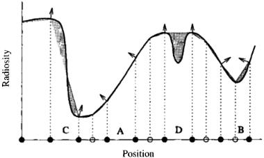
Figure 6.26: Cohen’s subdivision criterion based on the difference between nodal values results in the subdivision of element A, although linear interpolation provides a good approximation in this case. (Added nodes due to the subdivision are indicated by hollow circles.) The local minimum at D is also missed.

[61] compare the radiosities of an element and its neighbors . If these differ in value by more than a user-specified tolerance, the element is subdivided. For the constant elements, this is essentially equivalent to estimating the local error by comparing the piecewise constant approximation to linear interpolation through the same nodes and nodal values.

For rendering, however, Cohen uses linear interpolation. With respect to linear interpolation, this subdivision criterion is better characterized as a heuristic designed to produce smaller elements in regions where the radiosity is highly variable. This heuristic usually produces acceptable results, although it tends to oversubdivide where the gradient is high but constant. Since linear interpolation is a reasonable approximation for this case, subdividing has little effect on the error (see Figure 6.26.)

This heuristic may also fail to identify elements that should be subdivided. In Figure 6.26 the nodes bounding an element containing a local minimum (letter D in the figure) happen to have almost the same value. The heuristic fails in this case, since the nodal values alone do not provide enough information about the behavior of the function on the element interior. This difficulty is common to all types of error estimators and algorithm make efforts of varying sophistication to characterize the function between nodes.

For example, Vedel and Puech [242] use the gradient at the nodes as well as the function value. Elements are subdivided if the gradients at the element nodes vary by more than a certain tolerance (see Figure 6.27). This criterion avoids subdividing elements unnecessarily where the gradient is high but constant (letter

Radiosity and Realistic Image Synthesis	160
Edited by Michael F. Cohen and John R. Wallace

CHAPTER 6. RENDERING

6.3 AUTOMATIC MESHING ALGORITHMS

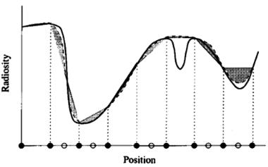
Figure 6.27: Gradient-based subdivision criterion. Nodes added due to adaptive subdivision are indicated by hollow circles.

A of Figure 6.27). It may also detect a local minimum within an element whose nodal values happen to be similar (letter B of Figure 6.27). However, the criterion is not foolproof. Letter C of Figure 6.27 shows a situation that might occur when a penumbra falls entirely within an element. The gradients at the nodes spanning the element happen to be equal and the element is not subdivided.

A more stringent criterion can be constructed that uses both the nodal values and gradients. An algorithm based on this approach might first compare gradients at the nodes. If the gradients vary by too much, the element is subdivided. Otherwise, the gradient at the nodes is compared to the slope of the plane determined by the nodal values. If they are inconsistent, the element is subdivided. This criterion correctly identifies the element at letter C in Figure 6.27, although it does not identify the case indicated by the letter D.

Higher-Order Subdivision Criteria

Vedel and Puech describe a test-bed system that estimates local error based on a higher-order (bicubic) interpolant over rectangular elements [242]. The local error estimate is provided by the L2 norm of the difference between bilinear and bicubic interpolation over an element (see Figure 6.28). This integral is evaluated in closed form as a function of the radiosities and gradients at the element nodes.

In comparing the higher-order error estimate to value—and gradient-based criteria for several simple cases, Vedel and Puech find the bicubic interpolation estimate to be the most accurate of the three when the radiosity is slowly varying. However, it fails to identify elements across which the radiosity is

Radiosity and Realistic Image Synthesis	161
Edited by Michael F. Cohen and John R. Wallace

CHAPTER 6. RENDERING

6.3 AUTOMATIC MESHING ALGORITHMS

Figure 6.28: Estimation of error by comparing linear and cubic interpolation. The gray area represents the estimated error. Nodes that will be added due to adaptive subdivision are indicated by hollow circles.

changing very rapidly, for example, where the element contains a sharp shadow boundary. In this case, the simple comparison of values does better, although as expected, it tends to oversubdivide in other regions. Vedel and Puech conclude that the complexity of the bicubic method is not justified, and they suggest simply comparing both radiosities and gradients.

Estimation Using the Residual

All of the methods described so far ultimately fail at some point because the nodes can never be relied on to completely characterize the behavior of the function elsewhere in the element. A local minimum or maximum can fall entirely within an element without affecting the function or its derivatives at the nodes, as is the case for the local minimum at letter D in Figure 6.26. Small shadows are often missed for this reason, with one common result being the appearance of floating furniture in radiosity images (see the artifact labeled B in Figure 6.3(b).)

In such cases, the only solution is to evaluate the function inside the element. One approach is to evaluate the radiosity equation at one or more points within the element and compare the results to the interpolated values. This is equivalent to estimating the residual, (described in section 6.1.3.)

Lischinski et al. [153] have used this technique for one-dimensional elements in a “flatland” radiosity implementation. In [154] they generalize this approach to two-dimensional elements by evaluating the radiosity at the centroid of the element and comparing it to the interpolated value at the same location (see

Radiosity and Realistic Image Synthesis	162
Edited by Michael F. Cohen and John R. Wallace

CHAPTER 6. RENDERING

6.3 AUTOMATIC MESHING ALGORITHMS

Figure 6.29: Estimation of error by computing the residual at element centers. The hollow circles represent interpolated values and the solid circles the computed value. The residual is the difference between the two.

Figure 6.29). The error at the centroid is assumed to be the maximum error for the element. This approach can thus be viewed as estimating the L∞ norm. This technique is independent of the interpolation order (quadratic interpolation was used by Lischinski et al.).

Of course, evaluating the error at the centroid is not guaranteed to catch every case. In Lischinski’s implementation, mesh boundaries corresponding to discontinuities in the radiosity function or its derivatives are specified a priori. Thus, a posteriori adaptive subdivision is required to refine the mesh only within regions over which the radiosity function is relatively smooth and well behaved, in which case checking the error at the centroid will generally produce good results.

Campbell [42] describes a more systematic approach to determining the behavior of the function on the interior. This is particularly useful when the radiosity function cannot be assumed to be smooth. Campbell’s criterion for subdivision uses the difference between the maximum and minimum radiosities over the entire element, not just at the nodes. Elements that require subdivision are split perpendicularly to the line connecting the maximum and minimum points. Thus, Campbell's algorithm depends on a systematic search for the extrema, which is achieved using standard optimization techniques.

Since Campbell's algorithm computes shadow boundaries a priori, it can identify fully lit regions and treat them differently from penumbra regions, which are more complex. For fully lit regions Campbell computes the gradient at the nodes analytically by differentiating the point-polygon form factor equation. This allows the use of optimization techniques that take advantage of gradient

Radiosity and Realistic Image Synthesis	163
Edited by Michael F. Cohen and John R. Wallace

CHAPTER 6. RENDERING

information to accelerate the search. In addition, for a fully lit region there can be only one local maximum on the interior of the element due to a given constant diffuse source.

For regions within the penumbra the gradient cannot be computed analytically and no assumptions can be made about the number of local extrema. In this case global optimization is performed using the Multistart method. A grid is laid over the region and the function is evaluated at a random point inside each grid cell. Cells whose neighbors are either all greater or all lesser in value than the cell itself provide the starting point for local optimization.

None of the error criteria that have been described in these sections can guarantee that small features will be found. This is one advantage of discontinuity meshing (discussed in Chapter 8), which locates critical shading boundaries a priori based on the model geometry. Within regions bounded by discontinuities, the radiosity function is reasonably well behaved, and simple error estimators are more reliable.

Computing the Gradient

A number of error estimators require the gradient of the radiosity at the nodes. Campbell points out that the analytic expression for the form factor between a differential area and a constant, unoccluded polygonal element is continuous and differentiable [42]. The expression can thus be symbolically differentiated to provide an analytic formula for the gradient at unoccluded nodes. However, the gradient is difficult or impossible to compute analytically in the presence of occlusion and is actually undefined at certain discontinuity boundaries.

Numerical differencing can also be used to compute partial derivatives. If the nodes fall on a regular grid, a first-order estimate of the partial derivative along grid lines can be made by comparing a nodal value with that of its neighbors. This estimate can be computed using forward or backward differencing, given by

B	=	B(xi ) − B(xi −1 )	(6.10)
x		xi − xi −1

where xi and xi–1are neighboring nodes. Central differencing can also be used, given by

B	=	B(xi +1 ) − B(xi −1 )	(6.11)
x		xi +1 − xi −1

If the mesh is irregular, the tangent plane at the node can be estimated using a least-squares fit of a plane to the values at the node and its immediate neighbors. (The contouring literature is a good source for techniques of this kind [257].) The accuracy of these techniques depends on the spacing between nodes.

Radiosity and Realistic Image Synthesis	164
Edited by Michael F. Cohen and John R. Wallace

CHAPTER 6. RENDERING

6.3 AUTOMATIC MESHING ALGORITHMS

Figure 6.30: Two different subdivisions of the same element. The upper right subdivision does not reduce the overall error of the approximation.

Another option is to perform extra function evaluations at points in the neighborhood of the node. For example, Salesin et al. [203] use quadratic triangular elements having nodes at the midpoint of each edge. To compute the gradient, a quadratic curve is fit to the values of the three nodes along each edge. The tangents of the two parabolas intersecting a given corner node determine a tangent plane at the node, and thus the gradient. This technique is described in more detail in section 9.2.2.

Ward describes a technique useful for methods that compute the irradiance at a point by sampling the visible surfaces over the entire hemisphere above the point, as in the hemicube [253]. The method was developed in the context of Ward’s Radiance lighting simulation system, which does not use radiosity. However, a full-matrix (gathering) radiosity solution using the hemicube or similar method for computing form factors is equally amenable to Ward's technique, although as yet no radiosity implementations have taken advantage of it.

6.3.4 Deciding How to Subdivide

Identifying elements that require subdivision is only the first step. The goal in identifying elements for subdivision is to reduce the local error for those

Radiosity and Realistic Image Synthesis	165
Edited by Michael F. Cohen and John R. Wallace

CHAPTER 6. RENDERING

6.3 AUTOMATIC MESHING ALGORITHMS

elements, but the actual reduction in error will depend~ on how the elements are subdivided. For example, in Figure 6.30, two ways of subdividing an element are compared. In one case, the error is reduced significantly, while in the other it is not reduced at all.

Subdividing intelligently requires some estimate of the behavior of the function inside the element. Campbell’s optimization approach, described in the previous section, is one of the few algorithms that attempts to obtain and use this information. Campbell searches for the maximum and minimum points on the interior of the element. The element is then subdivided on a boundary perpendicular to the line connecting the maximum and minimum points. The flexibility required to subdivide in this way places demands on the actual subdivision algorithm. Campbell chooses a BSP-tree based approach for this reason.

Airey [5] and Sturzlinger [227] note a useful technique for the special case of subdividing rectangles into triangles. The edge created to split the rectangle should connect the nodes with the most similar radiosities, since this produces the greatest reduction in the variation between the nodes of each of the resulting elements. Schumaker [207] discusses a generalization of this approach in which the behavior of the approximation is incorporated into the quality metric used during triangulation of the set of nodes. This more general approach has not yet been applied to radiosity, however.

In the absence of knowledge about the function behavior, the best that can be done is to subdivide uniformly. This is the approach taken by most existing adaptive subdivision algorithms. The resulting subdivision will depend on the particular subdivision algorithm. One common approach is to subdivide elements into four similarly shaped elements, generating a quadtree subdivision hierarchy. If the elements are triangles, another approach is to subdivide elements, by inserting nodes and adding new edges. These and a wide variety of other subdivision algorithms are surveyed in Chapter 8, with some discussion of how they can be applied to adaptive subdivision.

Radiosity and Realistic Image Synthesis	166
Edited by Michael F. Cohen and John R. Wallace

CHAPTER 7. HIERARCHICAL METHODS

Chapter 7

Hierarchical Methods

The meshing strategies surveyed in the previous chapter are designed to reduce the computational cost of the radiosity solution by minimizing the number of elements in the mesh. The solution cost depends strongly on the number of elements, since solving the discrete radiosity equation requires computing an interaction between every pair of elements. Thus, the cost of the radiosity solution appears to be inherently O(n2) in the number of elements. Each of these O(n2) relationships involves evaluating the form factor integral (the subject of Chapter 4) and is thus expensive to compute. Hence, the goal of the meshing strategies outlined in the previous chapter is to minimize the number of elements while maintaining accuracy.

The subject of this chapter is an alternative approach to reducing the computational cost of the radiosity algorithm. This approach keeps the same number of elements, instead attempting to reduce the number of individual relationships, or form factors, that have to be computed. For example, two groups of elements separated widely in space might reasonably have the total interaction between all pairs of individual elements represented by a single number computed once for the entire group. Attaining this goal involves developing a hierarchical subdivision of the surfaces and an associated hierarchy of interactions. The hierarchy will provide a framework for deriving interactions between groups of elements, which will result in computing many fewer than O(n2) interactions. In fact, it will turn out that only O(n) form factors are required to represent the linear operator K to within a desired error tolerance.

This chapter is divided into three major sections. The first two sections describe hierarchical subdivision techniques that minimize the number of form factors to be computed by grouping elements together. The first section assumes that constant basis functions have been selected to approximate the radiosity function. The section begins with a description of a two-level, patch-element hierarchy and continues with the generalization of the basic hierarchical approach, resulting in an O(n) algorithm. The second section then describes an alternate way of approaching the same goal, in which the hierarchical algorithms are derived in terms of hierarchical basis functions. One such class of basis func-

Radiosity and Realistic Image Synthesis	167
Edited by Michael F. Cohen and John R. Wallace

CHAPTER 7. HIERARCHICAL METHODS

7.1 A PHYSICAL EXAMPLE

Figure 7.1: Room with a desk and wall.

tions, known as wavelets, will be used to represent the kernel of the radiosity function at variable levels of detail. This formulation will provide a framework for incorporating higher order basis functions into hierarchical algorithms.

The third section of the chapter introduces an adjoint to the radiosity equation that allows the importance of a particular element to the final image to be determined. The combined radiosity equation and its adjoint will provide yet another means to reduce greatly the computational complexity for complex environments, in the case where only one, or a few, views are required.

I.Hierarchical Subdivision

7.1A Physical Example

The basic physical intuition behind hierarchical solution methods is straightforward. Imagine a room containing a table on which are placed several small objects (see Figure 7.1). Light reflected from the table top contributes some illumination to the wall. Intuitively, however, the shading of the wall does not depend significantly on the small details of the illumination leaving the table top. If the objects on the table are rearranged so that the shadows on the table are slightly altered, the shading of the wall does not change significantly.

Representing the contribution of the table top to the wall by a single average value will give a similar result to computing individual contributions from many small elements on the table top. This is because ideal diffuse reflection effectively averages the light arriving over an incoming solid angle. If the solid angle is not too great, as is the case when a source is far away relative to its

Radiosity and Realistic Image Synthesis	168
Edited by Michael F. Cohen and John R. Wallace