Baer M., Billing G.D. (eds.) - The role of degenerate states in chemistry (Adv.Chem.Phys. special issue, Wiley, 2002)

232	r. englman and a. yahalom

In the excited states for the same potential, the log modulus contains higher order terms in x (x3, x4, etc.) with coefficients that depend on time. Each term can again be decomposed (arbitrarily) into parts analytic in the t half-planes, but from elementary inspection of the solutions in [261,262] it turns out that every term except the lowest [shown in Eq. (59)] splits up equally (i.e., the f ’s are just 1=2) and there is no contribution to the phases from these terms. Potentials other than the harmonic can be treated in essentially identical ways.

F.Consequences

The following theoretical consequences of the reciprocal relations can be noted:

1.They unfold a connection between parts of time-dependent wave functions that arises from the structure of the defining equation (2) and some simple properties of the Hamiltonian.

2.The connection holds separately for the coefficient of each state component in the wave function and is not a property of the total wave function (as is, e.g., the ‘‘dynamical’’ phase [9]).

3.The relations pertain to the fine, small-scale time variations in the phase and the log modulus, not to their large-scale changes.

4.One can define a phase that is given as an integral over the log of the amplitude modulus and is therefore an observable and is gauge invariant. This phase [which is unique, at least in the cases for which Eq. (9) holds] differs from other phases, those that are, for example, a constant, the dynamic phase or a gauge-transformation induced phase, by its satisfying the analyticity requirements laid out in Section I.C.3.

5.Experimentally, phases can be obtained by measurements of occupation probabilities of states using Eq. (9). (We have calculationally verified this for the case treated in [264].)

6.Conversely, the implication of Eq. (10) is that a geometrical phase appearing on the left-hand side entails a corresponding geometric probability change, as shown on the right-hand side. Geometrical decay probabilities have been predicted in [162] and experimentally tested in [265].

7.An important ingredient in the analysis has been the positions of zeros ofðx; tÞ in the complex t plane for a fixed x. Within quantum mechanics the zeros have not been given much attention, but they have been studied in a mathematical context [257] and in some classical wave phenomena ([266] and references cited therein). Their relevance to our study is evident since at its zeros the phase of ðx; tÞ lacks definition. Future theoretical work shall focus on a systematic description of the location of zeros. Further, practically oriented work will seek out computed or

complex states of simple molecular systems

233

experimentally acquired time dependent wave functions for tests or application of the present results.

8.Finally, and probably most importantly, the relations show that changes (of a nontrivial type) in the phase imply necessarily a change in the occupation number of the state components and vice versa. This means that for time-reversal-invariant situations, there is (at least) one partner state with which the phase-varying state communicates.

IV. NON-LINEARITIES THAT LEAD TO MULTIPLE

DEGENERACIES

In previous sections, we treated molecules and other localized systems in which a linear electron-nuclear coupling resulted in a single degeneracy, or ci of the electronic potential energy surfaces. A notable, symmetry-caused example of this is the linear E E Jahn–Teller effect (a pair of degenerate electronic states, that can happen under trigonal or higher symmetry, which is coupled to two energetically degenerate displacement modes) [47,157,267]. Still, some time ago nonlinear coupling was also considered within the E E case in [268,269] and subsequently in [256]. Such coupling can result in a more complex situation, in which there is a quadruplet of ci’s, such that one ci is situated at the origin of the mode coordinates (as before) and three further ci’s are located farther outside in the plane, at points that possess trigonal symmetry.

As of late, nonlinear coupling has become of increased interest, partly through evidence for a weak linear coupling in the metallic cluster Na3 [52,270] (computations of vibrational levels in a related molecule Li3 were performed in [271,272]), and partly by attempts to computationally locate ci’s in the potential energy landscape with a view to estimate their effect on intersurface, nonadiabatic transitions [273]. The method used in the last reference was based on the acquisition of the geometric phase by the total function as a ci is circled [9,158,159,274]. Independently, the authors of [54] theoretically found a causal connection between the number of ci effectively circled (one or four) and the important question of the nature of the ground state. They showed that, contrary to what had been widely thought before, the ground state may be either a vibronic doublet or a singlet, depending on the distance (which is a function of the parameters in the vibronic Hamiltonian) of these trigonal ci’s from the centre. (A similar instance of ‘‘quantum phase transition’’ was noted for a threefold degenerate system in [275] and, earlier, for an icosahedral system, in [276]).

In a different field, location, and characteristics of ci’s on diabatic potential surfaces have been recognized as essential for the evaluation of dynamic parameters, like non-adiabatic coupling terms, needed for the dynamic and

234	r. englman and a. yahalom

static properties of some molecules ([193,277–280]). More recently, pairs of ci’s have been studied [281,282] in greater detail. These studies arose originally in connection with a ci between the 12A0 and 22A0 states found earlier in computed potential energy surfaces for C2H in Cs symmetry [278]. Similar ci’s appear between the potential surfaces of the two lowest excited states 1A2 and 1B2 in H2S or of 2B2 and 2A1 in Al H2 within C2v symmetry [283]. A further, closely spaced pair of ci’s has also been found between the 32A0 and 42A0 states of the molecule C2H. Here the separation between the twins varies with the assumed C C separation, and they can be brought into coincidence at some separation [282].

In this section we investigate the phase changes that characterize the double and trigonal (or cubic) ci’s. We shall find that the Berry phases upon circling around all the ci’s can take the values of 0 or 2Np (where N is an integer). It can be shown that the different values of N can be made experimentally observable (through probing the state populations after inducing changes in the amplitudes of the components), in a way that is not marred by the fast oscillating dynamic phase. Apart from the results regarding the integer N in the Berry phase, the difference between our approach to the phase changes and those in some previous works, especially in [273,283], needs to be noted. While these consider the topological phase belonging to the total wave packet, we continue in the spirit of the previous Section III and treat the open phase belonging to a single component of the wave packet. (For the topological, full-cycle phase the two are equivalent, but not for the open phase, that is present at interim stages.) Explicitly, we write the (in general) time (t)-dependent molecular wave function

ðtÞ as a superposition of (diabatic) electronic states wk as

X

ðtÞ ¼ akðtÞwk ð65Þ

k

where the amplitudes ak are functions of the nuclear coordinates. In Section III, we developed and used the reciprocal relations between the phases (arg ak) and the (observable) moduli (jakj).

We also describe a ‘‘tracing’’ method to obtain the phases after a full cycling. We shall further consider wave functions whose phases at the completion of cycling differ by integer multiples of 2p (a situation that will be written, for brevity, as ‘‘2Np’’). Some time ago, these wave functions were shown to be completely equivalent, since only the phase factor (viz., eiPhase) is observable [156]; however, this is true only for a set of measurements that are all made at instances where the phase difference is 2Np. We point out simple, necessary connections between having a certain 2Np situation and observations made prior to the achievement of that situation. The phase that is of interest in this chapter is the Berry phase of the wave function [9], not its total phase, though this distinction will not be restated.

complex states of simple molecular systems

235

A.Conical Intersection Pairs

We treat this case first, since it is simpler than the trigonal case. The molecular displacements are denoted by x and y (with suitable choice of their origins and of scaling). Then, without loss of generality we can denote the positions of the ci pairs in Cartesian coordinates by

x ¼ 1 y ¼ 0

ð66Þ

or, in polar coordinates, where x ¼ q cos f, y ¼ q sin f, by

q ¼ 1 f ¼ 0; p

ð67Þ

To obtain potential surfaces for two electronic states that will be degenerate at these points, we write a Hamiltonian as a 2 2 matrix in a diabatic representation in the following form:

H

x; y

Þ ¼

K

ðx2 1Þ

yf ðxÞ

ð

yf ðxÞ

ðx2 1Þ

¼

K

ðq2 cos 2f 1Þ

q sin f f ðq cos fÞ

¼

H

q;

fÞ

ð

68

Þ

q sin f f ðq cos fÞ

ðq2 cos 2f 1Þ

ð

whose two eigenvalues are

q

E ðx; yÞ ¼ K ðx2 1Þ2 þ ½y f ðxÞ&2

q

¼ K ðq2 cos 2f 1Þ2 þ ½q sin f f ðqcos fÞ&2

¼ E ðq; fÞ

ð69Þ

For K, a (positive) constant and f ðxÞ a function that is nonzero at x ¼ 1, the Hamiltonian in Eq. (68) can be taken as a model that yields the postulated ci pairs, since the two eigenvalues coincide just at the points given by Eq. (66) or (67). There may be more general models that give the same two ci’s. (Note, however, that if f ðxÞ had a zero at x ¼ 1, the degeneracy of energies would not be conical.) We now make the above model more specialized and show that different values of the Berry phase can be obtained for different choices of f ðxÞ. For definiteness we consider specific molecular situations, but these are just instances of wider categories. (The notation of Herzberg [284] is used.)

1.1A1 and 2A2 States in C2v Symmetry (Exemplified by

1Að11Þ and 1Að12Þ in Bent HCH)

If the x coordinate represents a mode displacement that transforms as B1 (e.g., an asymmetric stretch of CH) and y transforms as A1 (a flapping motion of the

236 r. englman and a. yahalom

H2, this coordinate being the same as y in Fig. 169 of [284]), then f ðxÞ in Eq. (68) can be taken as a constant. Without loss of generality we put for this case f ðxÞ ¼ 1 and find that cycling adiabatically counterclockwise around the ci that is at ð 1; 0Þ induces (in the component that is unity at f ¼ 0) a topological phase of p, and that around ð1; 0Þ yields p. Cycling either fully inside or outside q ¼ 1 (the latter case encircling both ci’s), gives zero phase. We now describe a ‘‘continuous (phase-) tracing method’’ that obtains in an unambiguous way the phase of a real wave function. The alternative, ‘‘adiabatic cycling’’ method Section III gave the same phase change in terms of the evolution of the complex solution of the time-dependent Schro¨dinger equation in the extremely slow (adiabatic) limit. Other methods will be briefly referred to.

B.Continuous Tracing of the Component Phase

In this method, one notes that real-valued solutions of the time-independent Hamiltonian of a 2 2 matrix form can be written in terms of an yðf; qÞ, which is twice the ‘‘mixing angle,’’ such that the electronic component which is ‘‘initially’’ 1 is cos ½yðf; qÞ=2&, while that which is initially 0 is sin ½yðf; qÞ=2&. For the second matrix form in Eq. (68) (in which, for simplicity f ðxÞ ¼ 1), we get

q sin f	ð70Þ
yðf; qÞ ¼ arctan q2 cos 2f 1

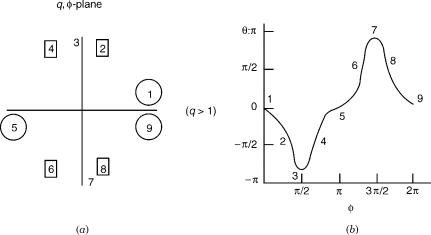
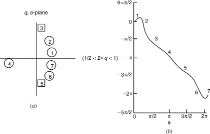
One can trace the continuous evolution of y (or of y=2) as f describes the circle q ¼ constant. This will yield the topological phase (as well as intermediate, open-path phase during the circling). We illustrate this in the next two figures for the case q > 1 (encircling the ci’s).

In Figure 2a several important stages in the circling are labeled with Arabic numerals. In the adjacent Figure 2b the values of yðf; qÞ are plotted as f increases continuously. The labeled points in the two Figures correspond to each other. (The notation is that points that represent zeros of tan y are marked with numbers surrounded by small circles, those that represent poles are marked by numbers placed inside squares, other points of interest that are neither zero nor poles are labeled by free numbers.) The zero value of the topological phase (y=2) arises from the fact that at the point 3 (at which f ¼ p=2), y retraces its values, rather than goes on to decrease.

1.A1 and B2 States in C2v Symmetry (Exemplified by

2A1 and 2B2 in AlH2 [285])

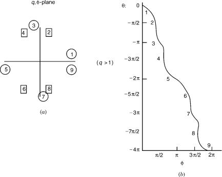
Symmetry considerations forbid any nonzero off-diagonal matrix elements in Eq. (68) when f ðxÞ is even in x, but they can be nonzero if f ðxÞ is odd, for example, f ðxÞ ¼ x. (Note that x itself transforms as B2 [284].) Figure 3 shows the outcome for the phase by the continuous phase tracing method for cycling

complex states of simple molecular systems

237

Figure 2. Phase tracing for the case of 1A1 and 2A2 states in C2v symmetry: (a) The left-hand side shows the labels for the significant stages during the circling the (q; f) plane. In this and the following figures, numbers in circles represent the positions of zeros in the argument of the arctan in the expression of the angle [Eq. (70)], numbers in squares are poles and free numbers are other significant stages in the circling. (b) The angle y in Eq. (70) as a function of the circling angle. The numbers correspond to those on the adjacent part (a) of the figure. (Note: The angle y is defined as twice the transformation or mixing angle.) The circling is with q > 1, namely, outside the ci pair.

outside the ci’s (q > 1). The difference between the present case and the previous one [in which f ðxÞ was an even function of x] is that now, in the second half of circling in the q; f plane, the wave function component angle y does not retrace its path, but goes on decreasing. [It is interesting to remark here on an analogy between the present results and the well-known results of contour integration in the complex z plane. An integration of ðz2 1Þ 1 over a path that encircles the two poles of the function gives zero result, but the same path integration of zðz2 1Þ 1, gives 2pi. However, the analogy does not work fully. Thus, a simple multiplication of the integrand by a positive constant alters the residues, but not the phase.]

However, the resulting Berry phase of 2p depends on (1) having reached the adiabatic limit and (2) circling well away from the ci’s; that is, it is necessary that the circling shall be done with a value of q that is either or 1. A contrary case not satisfying these conditions, for example, when either q < 3 or K < 60, would give a Berry phase of 4p, 6p, . . ., or a number N 2; 3; . . .

rather than 1, as might have been expected. What is perhaps remarkable is that even in the not quite adiabatic or not very large q cases, N (though plainly different from 1) is still close to being an integer. More study may be needed on this result, especially in view of the possibility of observable consequences of

238	r. englman and a. yahalom

Figure 3. Phase tracing for circling outside the ci pair for the model in A1 and B2 states in C2v symmetry. The Berry phase (half the angle shown at the extremity of the figure) is here 2p.

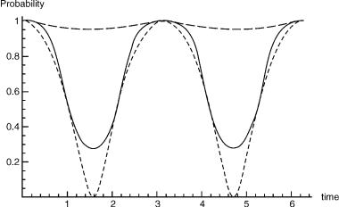
the value of N. The cases of ‘‘1A1 and 2A2 states in C2v symmetry’’ and of ‘‘A1 and B2 states in C2v symmetry’’ are, of course, inequivalent, since they arise from different Hamiltonians. Their nonequivalence results not only in different topological phases (zero and 2p), but in different state occupation probabilities. These are defined as the probabilities of the systems being in one of the states wk, of which the superposition in Eq. (65) is made up. In Figure 4, we show these probabilities as functions of time for systems that differ by their having different functions f ðxÞ in the off-diagonal positions of the Hamiltonian. The differences in the probabilities are apparent.

2.Trigonal Degeneracies

The simplest way to write down the 2 2 Hamiltonian for two states such that its eigenvalues coincide at trigonally symmetric points in ðx; yÞ or ðq; fÞ, plane is to consider the matrices of vibrational–electronic coupling of the E E Jahn– Teller problem in a diabatic electronic state representation. These have been constructed by Halperin, and listed in Appendix IV of [157], up to the third

complex states of simple molecular systems

239

Figure 4. Probabilities in different models during adiabatic circling around ci’s. The square moduli of component amplitudes as function of time are seen to be different for different models. Long-dashed lines: the model in 1A1 and 2A2 states in C2v symmetry for circling inside the ci’s. Full lines: the model in 1A1 and 2A2 states in C2v symmetry for circling outside the ci’s. Broken lines: the model in A1 and B2 states in C2v symmetry (with the ‘‘xy’’ off-diagonal matrix element) for circling outside the ci’s. In the latter model, circling inside the ci’s gives probabilities that would be indistinguishable from unity on the figure (and are not shown).

order in q. The first order or linear coupling in the displacement coordinates is of the well-known form (shown by the first term in the Hamiltonian presented below) and yields the familiar ci at the origin, q ¼ 0. When one adds to this the quadratic coupling, designated IðEÞ in Section IV.3 (A) of [157] and quoted below, one obtains three further, trigonally situated ci, namely, at either f ¼ 0; 2p=3, or f ¼ p; 4p=3, depending on whether the signs of the linear and quadratic couplings are the same or opposite. The distance of the trigonal ci’s from the origin varies with the relative magnitudes of the couplings: The higher the strength of the quadratic term, the nearer the trigonal ci are to the center. This was, of course, the physical basis of [54], in which a ground vibronic singlet state for strong quadratic coupling was found. The resulting Hamiltonian is of the form (to be compared with the two matrices in Eq. (68)):

H	x; y	Þ ¼	K	ðx 2kðx2 y2ÞÞ			y þ 4kxy
ð				y þ 4kxy	ðx 2kðx2 y2ÞÞ
		¼ K		q cos 2kq2 cos 2f		Þ		q sin f	þ	2kq2 sin 2f
				ðq sin ff 2kq2 sin 2f			ð	q cos f		2kq2 cos 2f
				þ							Þ
		¼ Hðq; fÞ									ð71Þ

240	r. englman and a. yahalom

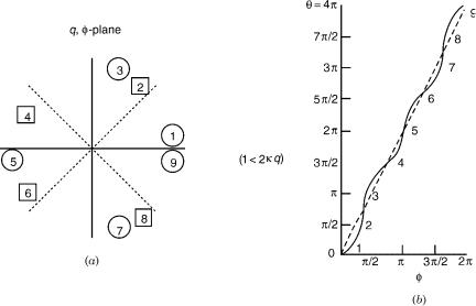
Figure 5. Phase tracing for the case of trigonal degeneracies when the circle encompasses all four ci’s and the Berry phase is 2p.

where k represents the ratio of the strength of the quadratic coupling to the linear one. The trigonal ci’s are at a distance q ¼ ð2kÞ 1, with angular positions as described above. Now by employing the continuous phase-tracing method introduced in Section I.D.1, one again obtains the graphs for the mixing angle. There are now three cases to consider, namely (1) for cycling that encloses all four ci’s ðq > ð2kÞ 1Þ the resulting phase acquired being now 2p (shown in Fig. 5). This is an even multiple of p, as expected for four ci’s [274], but differs from 4p (or from zero). Then (2) for intermediate radius cycling ðð2kÞ 1 > q > ð4kÞ 1Þ (which is shown in Fig. 6) that terminates with a Berry phase of p. Lastly, (3) for small radius cycling ðq < ð2kÞ 1Þ. The last case has also the Berry phase of p, but differs from the intermediate case (2), in that the initial increase is absent.

It might be asked what happens when one adds further couplings beyond the quadratic one? In the next higher order one finds a scalar cubic term of the form:

q3cos 3pI

ð72Þ

where I is the unit matrix. This gives rise to three trigonally aligned degeneracies ([157], Appendix IV). However, these are parabolic (touching) degeneracies, not conical intersections, and do not cause changes of sign in the wave function upon circling round them. Higher order terms (not listed in that appendix) can give rise

complex states of simple molecular systems

241

Figure 6. Phase tracing for the trigonal degeneracies. The drawings (which are explained in the caption to Fig. 3) are for intermediate radius (q) circling.

to additional ci’s of trigonal symmetry, but the strength of these terms is expected to be less and therefore the resulting ci’s will be farther outside, where they are without importance for low-lying states. Still, their presence is of interest for revealing the connection between the Berry angle and the number of ci’s circled and we shall presently obtain nonlinear coupling terms to an arbitrarily high power of q.

C.The Adiabatic-to-Diabatic Transformation (ADT)

Several years ago Baer proposed the use of a matrix A, that transforms the adiabatic electronic set to a diabatic one [72]. (For a special twofold set this was discussed in [286,287].) Computations performed with the diabatic set are much simpler than those with the adiabatic set. Subject to certain conditions, A is the solution of a set of first order partial differential equations. A is unitary and has the form of a ‘‘path-ordered’’ phase factor, in which the phase can be formally written as

R
ðR0	f IJ ðRÞ dR	ð73Þ

Here, the integrand is the off-diagonal gradient matrix element between adiabatic electronic states,

f IJ ðRÞ ¼ hIj$jJi

ð74Þ