Flow Cytometry - First Principles (Second Edition)

130

Flow Cytometry

Fig. 8.2. Compared with the narrow peak in the normal histogram at the upper left, it can be seen that a single peak with a wide coe½cient of variation (CV) or skewed pro®le may mask a near-diploid malignant cell line. In addition, an extra small peak at the 4C position may result from clumping of nuclei, cycling cells, or a true tetraploid abnormality. Data courtesy of Colm Hennessy.

grams (as a rule of thumb, <3% is good; >8% is not good). A wide CV might result from old and partially degraded material, from erratic ¯ow due to a partially clogged ¯ow ori®ce, from a ¯uctuating laser beam, from a sample that has been run too quickly (remember that widening of the core diameter within the sheath stream may lead to unequal illumination as particles stray from the center of the laser beam), from nuclei that have been unequally exposed to stain, or, ®nally, from abnormal cells with a DNA content quite close to that of the normal material. The sensitivity of the technique for detecting these near diploid abnormalities and thus for classifying tissue as euploid or aneuploid therefore depends on the cytometrist's ability to obtain narrow CVs in the normal controls.

Another problem concerning interpretation arises from the inconvenient fact that aneuploid tumors often have DNA content that is very close to double the amount found in normal cells. This amount is referred to as 4C or tetraploid. If we stop and think, we can immediately see why this might lead to problems in ¯ow analysis (see the small 4C peaks in Fig. 8.2). First of all, perfectly normal cells

DNA in Life and Death

131

with the 4C amount of DNA appear at certain phases in the cell cycle ( just before cell division); therefore, if normal dividing cells are present, a signi®cant number of particles may have double the 2C amount of DNA and will therefore appear in a peak at the tetraploid position. Second, remember that the ¯ow cytometer is poor in its ability to distinguish large particles from clumped particles. It is not surprising, then, that the cytometer is, in the same way, inadequate at distinguishing a nucleus with double the normal amount of DNA from two normal nuclei clumped together. Scientists and clinicians usually resort to adopting some threshold value for classi®cation purposes. For example, a sample with a 4C peak may be considered aneuploid only if the tetraploid peak contains more than 10% of the total number of nuclei counted; otherwise it will be considered normal on the assumption that about 10% of normal cells may appear in the tetraploid position owing to clumping and/or mitosis.

CELL CYCLE ANALYSIS

As mentioned above, normal cells will have more DNA than the 2C amount appropriate to their species at times when they are preparing for cell division. The cell cycle has been divided into phases (Fig. 8.3). Cells designated as being in the G0 phase are not cycling at all; cells in G1 are either just recovering from division or preparing for the initiation of another cycle; cells are said to be in S phase when they are actually in the process of synthesizing new DNA; cells in the G2 phase are those that have ®nished DNA synthesis and therefore possess double the normal amount of DNA; and cells in M phase are in mitosis, undergoing the chromosome condensation and organization that occur immediately before cytokinesis (resulting in the production of two daughter cells, each with the 2C amount of DNA). A DNA ¯ow histogram provides a snapshot of the proportion of different kinds of nuclei present at a particular moment. If we look at the DNA content of cells that are cycling (not resting), we will ®nd some nuclei with the 2C amount of DNA (either G0 or G1 cells), some nuclei with the 4C amount of DNA (G2 or M cells), and some nuclei with di¨erent amounts of DNA that span the range between these 2C and 4C populations (Fig. 8.4). A theoretical histogram distribution would look like Figure 8.5. Figure 8.6 shows an example of

132	Flow Cytometry

Fig. 8.3. The four successive phases of a typical mammalian cell cycle. From Alberts et al. (1989).

Fig. 8.4. Schematic illustration of the generation of a DNA distribution from a cycling population of cells. From Gray et al. (1990).

DNA in Life and Death

133

Fig. 8.5. The theoretical histogram generated from the sampling of a population of cycling cells.

DNA ¯ow histograms that result from the propidium iodide staining of cells taken from a culture before and after they have been stimulated to divide.

The traditional method for analyzing cell division involves measuring the amount of DNA being synthesized in a culture by counting the radioactivity incorporated into DNA when the dividing cells are given a 6 h pulse with tritiated thymidine. The DNA histogram resulting from ¯ow cytometric analysis o¨ers an alternative to this technique. By dividing the histogram up with four markers, we can delineate nuclei with the 2C amount of DNA, those with the 4C amount of DNA, and those with amounts of DNA between the two delineated regions and therefore caught in the process of synthesizing DNA. The nuclei making DNA and showing up between the two peak regions should in some way correlate with the values obtained for DNA synthesis based on the uptake of tritiated thymidine. The values are not directly convertible one to the other: The radioactive method re¯ects the total amount of DNA being synthesized and will give higher values when more cells are present, whereas the ¯ow method measures the proportion of cells that are in the process of making DNA and will not be a¨ected by increases in the total number of cells. In addition, the radioactive method will give higher values if there is a signi®cant amount of DNA repair going on,

134

Flow Cytometry

Fig. 8.6. DNA histograms from lymphocytes stimulated to divide.

whereas the ¯ow method will give higher values if a proportion of cells are blocked in S phase. However, with these provisos, ¯ow cytometry does o¨er a rapid and painless (nonradioactive) method for looking at cell proliferation.

Having agreed on the general principle that ¯ow cytometry in conjunction with propidium iodide staining is an appropriate technology for analyzing cell proliferation, we have now to face the problem that the actual histogram has a certain width to the G0/G1 and to the G2/M peaks and does not look like our theoretical distribution; we have to decide where to place those four markers mentioned above so as to delineate correctly the three regions (2C, 4C, and S phase). In a scenario that may by now be familiar, what seemed like a straightforward question turns out to have a less than

DNA in Life and Death

135

straightforward answer. Because the 2C and 4C peaks in a ¯ow histogram have ®nite widths (remember the discussion about CV in the section on ploidy), it turns out to be rather di½cult to decide where the 2C (or G0/G1) peak ends and nuclei in S phase begin. Similarly, it is di½cult to know exactly where the distribution from nuclei in S phase ends and the spread from nuclei in G2 or M (4C amount of DNA) begins. In fact, there is no unambiguously correct point to place markers separating these three regions: The regions overlap at their extremes as a result of the inevitable nonuniformity of staining and illumination. The question therefore becomes not where to place the markers delineating the three cell cycle regions, but how many of the nuclei lurking under the normal spread of the 2C and 4C regions of the histogram are actually in S phase. Enter the mathematicians.

Algorithms based on sets of assumptions about the kinetics of cell division and the resulting shape of cell cycle histograms can be used to derive formulae for separating the contribution to the ¯uorescence distribution from our three separate cell cycle components. The algorithms range from the simple to the complex. They all seem to work reasonably well (that is, they all give similar and intuitively appropriate answers) when cell populations are well behaved. However, they all re¯ect the intrinsic limitations of using simplistic mathematical models for complex biological systems when cell populations grow too rapidly, are blocked in the cycle, or are otherwise perturbed. Bearing these limitations in mind, we can now look at four of the models used.

Figure 8.7 shows a DNA histogram derived from the propidium iodide staining of cells from a dividing culture. The simplest method for analyzing this histogram is the so-called peak re¯ect method whereby the shape of the G0/G1 peak is assumed to be symmetrically distributed around the mode. Given this assumption, the width of the peak, from the mode to the left (low ¯uorescence) edge is simply copied to the right (high ¯uorescence) edge; the same thing is done in reverse with the G2/M peak. Then everything in the middle between these two delineated regions is considered to be the result of S-phase cells.

A slightly more complex method for estimating the proportion of S-phase cells is called the rectangular approximation method. This method assumes that cells progress regularly through S phase and therefore that the proportion of cells at any given stage of DNA

136

Flow Cytometry

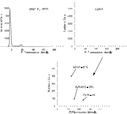
Fig. 8.7. Di¨erent mathematical algorithms for determining the contribution of S-phase nuclei to a DNA ¯ow histogram. Upper left and lower right from Dean (1987); upper right and lower left from Dean (1985).

synthesis is constant. When this method is used, the average number of cells in the middle region of the DNA histogram is evaluated, and the height of this region is then extrapolated in both directions, toward the 2C peak and toward the 4C peak. The rectangle derived from this evaluation is then ascribed to S-phase cells, and all the other cells are considered either G0/G1 or G2/M depending on whether they have higher or lower ¯uorescence than the middle point of the distribution.

The so-called S-FIT method and the sum-of-broadened-rectangles (SOBR) method both use more sophisticated mathematical assumptions to model the shape of the S-phase region of the histogram. A polynomial equation (S-FIT) or a series of broadened Gaussian dis-

DNA in Life and Death

137

tributions (SOBR) is derived that best ®ts the S-phase region of the histogram; then this derived shape is extrapolated toward the 2C and 4C peaks to estimate the contribution of S-phase cells within these regions.

One of the essential problems in assigning cells in a ¯ow histogram to certain stages of the cell cycle is that an aggregate or clump of two G0/G1 cells will have double the normal DNA content (remember our discussion of the problem in diagnosing tetraploid tumors) and will appear as if they are a single G2/M cell. One way of diagnosing a clumped sample is by looking for peaks at the 6C position (resulting from three nuclei together). If there are clumps of three cells, then, statistically, there will be even more clumps of two cells. DNA analysis software can estimate the doublet contribution to the tetraploid peak by using probability algorithms to extrapolate from the triplet peak at the 6C position. The software (Fig. 8.8, right hand plot) can then subtract out this doublet contribution and give a measure of the ``true'' number of G2/M cells.

As well as software-based aggregate subtraction, so-called pulse processing (or, more recently, digital) electronics can give us help in this task. In general, particles (cells or nuclei) give out signals that

Fig. 8.8. By looking at the peak at the 6C and 8C positions (aggregates of three and four cells), software algorithms use this information to estimate the contribution of clumps of two cells to the peak at the G2/M (4C) position. The graph at the right indicates the software estimation of these aggregated cells. The graph at the left indicates where these cells fall on a plot of signal area versus signal width.

138	Flow Cytometry

Fig. 8.9. The time that a ¯uorescence signal lasts (the signal width) depends primarily on the size of the laser beam (if the cell is smaller than the beam) or primarily on the size of the cell (if the cell is larger than the beam). From Peeters et al. (1989).

last, in time, just as long as it takes for the entire particle to move through the laser beam. What this means is that particles with diameters smaller than the laser beam all give out signals that last approximately the same length of time (dependent primarily on the laser beam width in the direction of ¯ow and on the stream velocity); this is a traditional method of ¯ow analysis. However, it is apparent that larger particles (or small particles in a very narrow laser beam) will give out signals whose time pro®les are related primarily to their own diameter (Fig. 8.9). Pulse processing or digital electronics involves analysis of the full pro®le of the ¯uorescence signal from a particle. This includes a measure of the signal's width (the time it takes for the cell to pass through the laser beam), its height (the maximum ¯uorescence during this passage), and its area (the total ¯uorescence emitted during this passage) (Fig. 8.10). One large (G2/M) nucleus will pass through a narrow laser beam more quickly than will two smaller aggregated nuclei of the same total DNA content; however, the G2/M nucleus will have greater ¯uorescence intensity when it is centered in the beam (assuming a narrow laser beam relative to the diameter of two cells). Therefore, the signal area is used as the DNA parameter in cell cycle analysis because it is most closely proportional to total DNA content of a cell, but the width and height characteristics of the resulting ¯uorescence signal can be stored as extra parameters and can be used to distinguish clumps

DNA in Life and Death

139

Fig. 8.10. Signal width, area, and height characteristics of light pulses as G1, G2, and two clumped G1 cells move through a narrow laser beam. Modi®ed from Michael Ormerod.

from single G2/M particles. This can help considerably in the interpretation of DNA histograms (Fig. 8.11).

Software algorithms for estimating the proportion of S-phase cells are approximations. They can be re®ned mathematically in the hope of better approaching the biological truth. A mathematical model will always, however, have trouble coping with a biological situation that is disturbed or contains mixed populations behaving in erratic

Fig. 8.11. Single cells (shown in the gates) can be distinguished from aggregates because single cells have lower signal widths and greater signal heights relative to their signal areas. The left plot is of data acquired on a Beckman Coulter cytometer; data in the right plot were acquired on a Becton Dickinson cytometer.