Advanced Wireless Networks - 4G Technologies

Table 3.25 Statistical models and parameters

Global parameters Gtot and Gk

Path loss

PL

20.4 log10(d/d0),

d ≤ 11 m

Shadowing

= −56 + 74 log10(d/d0), d > 11 m

G

tot LN (−PL; 4.3)

Decay constant

ε LN (16.1; 1.27)

Power ratio

r LN (−4; 3)

Local parameters Gk

Energy gains

Gk

(

G

k ; mk )

2

(τk )

mk

TN μm (τk );

σm

m Values

μm (τk ) = 3.5 −

τk

73

σm2 (τk ) = 1.84 −

τk

160

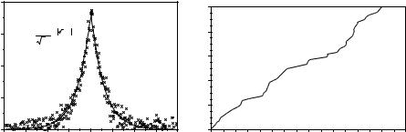
(a)

(b)

Figure 3.24 (a) The measured 49 local PDPs for an example room. (b) Simulated 49 local PDPs for an example room. (Reproduced by permission of IEEE [86].)

UWB CHANNEL MODEL 89

lth cluster, relative to Tl . The parameters and γ determine the intercluster signal level rate of decay and the intracluster rate of decay, respectively. The parameter is generally determined by the architecture of the building, while γ is determined by objects close to the receiving antenna, such as furniture. The results presented in Spencer et al. [95] make the assumption that the channel impulse response as a function of time and azimuth angle is a separable function, or

h (t, θ ) = h (t) h (θ )

(3.74)

from which independent descriptions of the multipath time-of-arrival and angle-of-arrival are developed. This is justified by observing that the angular deviation of the signal arrivals within a cluster from the cluster mean does not increase as a function of time.

The cluster decay rate and the ray decay rate γ can be interpreted for the environment in which the measurements were made. For the results, presented later in this section, at least one wall separates the transmitter and the receiver. Each cluster can be viewed as a path that exists between the transmitter and the receiver along which signals propagate. This cluster path is generally a function of the architecture of the building itself. The component arrivals within a cluster vary because of secondary effects, e.g. reflections from the furniture or other objects. The primary source of degradation in the propagation through the features of the building is captured in the decay exponent . Relative effects between paths in the same cluster do not always involve the penetration of additional obstructions or additional reflections, and therefore tend to contribute less to the decay of the component signals. Results for p(θ ) generated from the data in Cramer et al. [97] are shown in Figure 3.25. Interarrival times are hypothesized [95] to follow exponential rate laws, given by

p (Tl |Tl−1 ) = e− (Tl −Tl−1)

p Tkl Tk−1,l = λe−λ(Tl −Tl−1)

(3.75)

where is the cluster arrival rate and λ is the ray arrival rate. Channel parameters are summarized in Table 3.26.

(a)											(b)
	0.020										100
		Laplacian
		distribution:
	0.015	p(θ ) =	1	−	2θ / σ						80
			2σ e
p(θ)											60
	0.010										(%)
											cdf
											40
	0.005
											20
	0.000										0
	-180	-135	-90		-45	0	45	90	135	180	-180	-135	-90	-45	0	45	90	135	180
						θ (degrees)							Cluster angle-of-arrival relative to reference cluster

Figure 3.25 (a) Ray arrival angles at 1◦ of resolution and a best fit Laplacian density with σ = 38◦. (b) Distribution of the cluster azimuth angle-of-arrival, relative to the reference cluster. (Reproduced by permission of IEEE [97].)

90	CHANNEL MODELING FOR 4G
		Table 3.26	Channel parameters
Parameter UWB [97]		Spencer et al. [95] Spencer et al. [95]		Saleh and Valenzuela [94]
	27.9 ns	33.6 ns	78.0 ns	60 ns
γ	84.1 ns	28.6 ns	82.2 ns	20 ns
1/	45.5 ns	16.8 ns	17.3 ns	300 ns
1/λ	2.3 us	5.1 ns	6.6 ns	5 ns
σ	37◦	25.5◦	21.5◦	—

3.9.6 Path loss modeling

In this section we are interested in a transceiver operating at approximately 2 GHz center frequency with a bandwidth in excess of 1.5 GHz, which translates to sab-nanosecond time resolution in the CIRs.

3.9.6.1 Measurement procedure

The measurement campaign is described in Yano [98] and was conducted in a single-floor, hard-partition office building (fully furnished). The walls were constructed of drywall with vertical metal studs; there was a suspended ceiling 10 feet in height with carpeted concrete floor. Measurements were conducted with a stationary receiver and mobile transmitter; both transmit and receive antennas were 5 feet above the floor. For each measurement, a 300 ns time-domain scan was recorded and the LOS distance from transmitter to receiver was recorded. A total of 906 profiles were included in the dataset with seven different receiver locations recorded over the course of several days. Except for a reference measurement made for each receiver location, all successive measurements were NLOS links chosen randomly throughout the office layout that penetrated anywhere from one to five walls. The remainder of datapoints were taken in similar fashion.

3.9.6.2 Path loss modeling

The average pathless for an arbitrary TR separation is expressed using the power law as a function of distance. The indoor environment measurements show that, at any given d, shadowing leads to signals with a path loss that is log–normally distributed about the mean [99]. That is:

PL (d) = PL0 (d0) + 10N log	d	+ Xσ	(3.76)
	d0

where N is the pathloss exponent, Xσ is a zero mean log–normally distributed random variable with standard deviation σ (dB), PL0 is the free space path loss at reference distance, d0. Some results are shown in Figure 3.27.

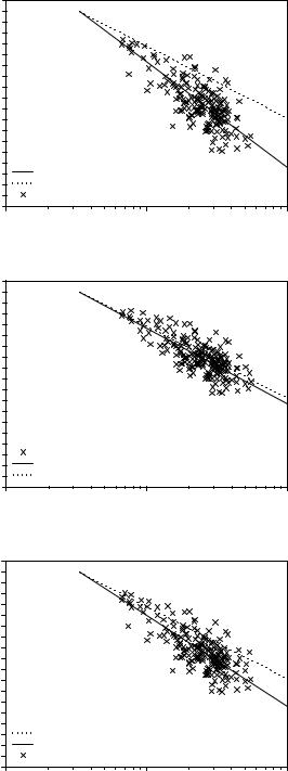
Assuming a simple RAKE with four correlators where each component is weighted equally, we can calculate the path loss vs distance using the peak channel impulse response (CIR) power plus RAKE gain, PLPEAK+RAKE, for each CIR, as shown in Figure 3.26(c). The

	3
	0
	-3
	-6
	-9		σN = 4.75 dB
	-12
	-15
(dB)	-18
	-21
PEAK	-24
	-27
PL
	-30
-	-33
	-36
	-39
	-42	Free space
	-45
	-48	N = 2.9
	-51	data
	-54
	100	101	102

Distance (feet)

		(a)
	3
	0
	-3
	-6		σN = 3.55 dB
	-9
	-12
(dB)	-15
	-18
	-21
TOTAL	-24
	-27
-PL	-30
	-33
	-36
	-39
	-42	Free space
	-45
	-48	N = 2.1
	-51	data
	-54
	100	101	102

Distance (feet)

		(b)
	3
	0
	-3
	-6		σN = 4.04 dB
	-9
	-12
(dB)	-15
	-18
PEAK+RAKE	-21
	-24
	-27
	-30
-PL
	-33
	-36
	-39
	-42	Free space
	-45
	-48	N = 2.5
	-51	data
	-54
	100	101	102

Distance (feet)

(c)

Figure 3.26 (a) Peak PL vs distance; (b) total PL vs distance; (c) peak PL + rake gain vs distance. (Reproduced by permission of IEEE [98].)

92 CHANNEL MODELING FOR 4G

τ (ns) RMS

50

45

40 σrms = 5.72 ns

35

30

25

20

15

10

5

0

100

101

102

Distance (feet)

				(a)
	50
	45
	40	σrms = 4.26 ns
	35
(ns)	30
RMS	25
τ
	20
	15
	10
	5
	0
	0	10	20	30	40	50	60

PLPEAK (dB)

(b)

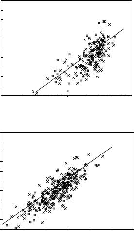
Figure 3.27 (a) The RMS delay spread vs distance; (b) RMS delay spread vs path loss. (Reproduced by permission of IEEE [98].)

exponent N obtained from performing a least-squares fit is 2.5 with a standard deviation of 4.04 dB. The results for delays are shown in Figure 3.27.

3.9.6.3 In-home channel

For the in-home channel Equation (3.76) can be also used to model path loss. Some results are shown in Table 3.27 [100–103]. Table 3.28 presents the results for delay spread in home channel [100].

REFERENCES 93

Table 3.27 Statistical values of the path loss parameters

		LOS			NLOS
	Mean		SD		Mean	SD
P L0 (dB)	47			51
N	1.7		0.3	3.5		0.97
σ (dB)	1.6		0.5	2.7		0.98

Table 3.28 Percentage of power contained in profile, number of paths, mean excess delay and RMS delay spread for 5, 10, 15, 20 and 30 dB threshold levels

			50 % NLOS					90 % NLOS
Threshold	Power %		L	τm(ns)	τRMS(ns)	Power %		L	τm(ns)	τRMS(ns)
5 dB	46.8		7	1.95	1.52	46.9		8	2.2	1.65
10 dB	89.2		27	7.1	5.77	86.5		31	8.1	6.7
15 dB	97.3		39	8.6	7.48	96		48	10.3	9.3
20 dB	99.4		48	9.87	8.14	99.5		69	12.2	11
30 dB	99.97		60	10.83	8.43	99.96		82	12.4	11.5

REFERENCES

[1]S. Glisic, Advanced Wireless Communications, 4G Technology. Wiley: Chichester 2004.

[2]K.I. Pedersen, P.E. Mogensen and B.H. Fleury, A stochastic model of the temporal and azimuthal dispersion seen at the base station in outdoor propagation environments,

IEEE Trans. Vehicle Technol., vol. 49, 2000, pp. 437–447.

[3]F. Frederiksen, P. Mogensen, K.I. Pedersen and P. Leth-Espensen, A software testbed for performance evaluation of adaptive antennas in FH GSM and wideband-CDMA, in Proc. 3rd ACTS Mobile Communication Summit, vol. 2, Rhodes, June 1998, pp. 430–435.

[4]A. Algans, K.I. Pedersen and P.E. Mogensen, Experimental analysis of the joint statistical properties of azimuth spread, delay spread, and shadow fading, IEEE J. Select. Areas Commun., vol. 20, 2002, pp. 523–531.

[5]D.C Cox, R. Murray and A. Norris, 800 MHz attenuation measured in and around sub-urban houses, AT&T Bell Lab. Tech. J., vol. 673, 1994.

[6]R.C. Bernhardt, Macroscopic diversity in frequency reuse systems, IEEE J. Select. Areas Commun., vol. 5, 1987, pp. 862–878.

[7]H. L. Bertoni, Radio Propagation for Modern Wireless System. Prentice-Hall: Englewood Cliffs, NJ, 2000.

[8]L. Correia, Wireless Flexible Personalised Communications-Cost 259 Final Report.

Wiley: New York, 2001.

[9]J. Winters, Optimum combining in digital mobile radio with cochannel interference

IEEE Trans. Vehicle Technol., vol. VT-33, 1984.

94CHANNEL MODELING FOR 4G

[10]K.I. Pedersen, P.E. Mogensen and B.H. Fleury, Spatial channel characteristics in outdoor environments and their impact on BS antenna system performance, in Proc. IEEE Vehicular Technology Conf. (VTC’98), Ottawa, May 1998, pp. 719–724.

[11]K.I. Pedersen and P.E. Mogensen, Evaluation of vector-RAKE receivers using different antenna array configurations and combining schemes, Int. J. Wireless Inform. Networks, vol. 6. 1999, pp. 181–194.

[12]V. Veen and K.M. Buckley, Bcamforming: a versatile approach to spatial filtering, lEEE Acoust., Speech Signal Processing (ASSP) Mag., vol, 5, 1988, pp. 4–24.

[13]J. Liberti and T. Rappaport, A geometrically based model for line-of-sight multipath radio channels, in Proc. IEEE Vehicular Technology Conf. (VTC 96), May 1996, pp. 844–848.

[14]M. Lu, T. Lo and J. Litva, A physical spatio-temporal model of multipath propagation channels, in Proc. IEEE Vehicular Technology Conf. (VTC 97), May 1997, pp. 810– 814.

[15]O. Nørklit and J.B. Andersen, Diffuse channel model and experimential results for antenna arrays in mobile environments, IEEE Trans. Antennas Propagat., vol. 96, 1998, pp. 834–840.

[16]C. Cheon, H.L. Bertoni and G. Liang, Monte Carlo simulation of delay and angle spread in different building environments, in Proc. IEEE Vehicular Technology Conf. (VTC’00), Boston, MA, vol.1, 20–28 September 2000, pp. 49–56.

[17]U. Martin, A directional radio channel model for densely built-up urban areas, in

Proc. European Personal Mobile Communications Conf. (EPMCC), Bonn, October 1997, pp. 237–244.

[18]M. Gudmundson, Correlation model for shadow fading in mobile radio systems, IEEE Electron. Lett., vol. 27, 1992, pp. 2126–2145.

[19]A. Mawira, Models fur the spatial correlation functions of the log-normal component of the variability of VHF/UHF field strength in urban environment, in Proc. Personal, Indoor and Mobile Radio Communications (PIMRC’92), London, 1992, pp. 436– 440.

[20]A. Gehring, M. Steinbauer, I. Gaspard and M. Grigat, Empirical channel stationarity in urban environments, in Proc. European Personal Mobile Communications Conf. (EPMCC), Vienna, February, 2001.

[21]T.B. Sørensen, Correlation model for shadow fading in a small urban macro cell, in Proc. Personal Indoor and Mobile Radio Communications (PIMRC’98), Boston, MA, 1998.

[22]Algorithms and antenna array recommendations, Public deliverable from European ACTS, TSUNAMI II Project, Deliverable code: AC020/AUC/A1.2/DR/P/005/bl, May 1997.

[23]Commission of the European Communities, Information technologies and sciences – digital land mobile radio communications, COST 207, 1998.

[24]P.A. Bello, Characterization of randomly time-variant linear channels, IEEE Trans. Commun. Syst., vol. CS-11, 1963, pp. 360–393.

[25]J.A. Fessler and A. Hero, Space-alternating generalised expectation-maximization algorithm, IEEE Trans. Signal Processing, vol. 42, 1994, pp. 2664–2677.

[26]B.H. Fleury, M. Tschudin, R. Heddergott, D. Dahlhaus and K. I. Pedersen, Channel parameter estimation in mobile radio environments using the SAGE algorithm, IEEE J. Select. Areas Commun., vol. 17, 1999, pp. 434–450.

REFERENCES 95

[27]K.I. Pedersen, B.H. Fleury and P.E. Mogensen, High resolution ot electromagnetic waves in time-varying radio channels, in Proc. Int. Symp. Personal, Indoor and Mobile Radio Communications (PIMRC’97), Helsinki, September 1997, pp. 650– 654.

[28]K.I. Pedersen, P.E. Mogensen , B.H. Fleury, F. Frederiksen and K. Olesen, Analysis of time, azimuth and doppler dispersion in outdoor radio channels, in Proc. ACTS Mobile Communication Summit ’97, Aalborg, October 1997, pp. 308–313.

[29]M. Hata, Empirical formula for propagation loss in land mobile radio service, IEEE Trans. Vehicle Technol., vol. VT-29, 1980, pp. 317–325.

[30]L.J. Greenstein, V. Erceg, Y.S. Yeh and M.V. Clark, A new path-gain/delay-spread propagation model for digital cellular channels, IEEE Trans. Vehicle Technol., vol. 46, 1997, pp. 477–485.

[31]M. Toeltsch, J. Laurila, K. Kalliola, A.F. Molisch, P. Vainikainen and E. Bonek, Statistical characterization of urban spatial radio channels, IEEE J. Select. Areas Commun., vol. 20, no. 3, 2002, pp. 539–549.

[32]R. Roy, A. Paulraj and T. Kailath, ESPRIT – a subspace rotation approach to estimation of parameters of cisoids in noise, IEEE Trans. Acoust., Speech, Signal Process., vol. 32, 1986, pp. 1340–1342.

[33]M. Zoltowski, M. Haardt and C. Mathews, Closed-form 2-D angle estimation with rectangular arrays in element space or beamspace via unitary ESPRIT, IEEE Trans. Signal Process., vol. 44, 1994, pp. 316–328.

[34]M. Haardt and J. Nossek, Unitary ESPRIT: how to obtain an increased estimation accuracy with a reduced computational burden, IEEE Trans. Signal Process., vol. 43, 1995, pp. 1232–1242.

[35]S.C. Swales, M. Beach, D. Edwards and J.P. McGeehan, The performance enhancement of multibeam adaptive base-station antennas for cellular land mobile ratio systems, IEEE Trans. Vehicle Technol., vol. 39, 1990, pp. 56–67.

[36]R.B. Ertel, P. Cardieri, K.W. Sowerby, T.S. Rappaport and J.H. Reed, Overview of spatial channel models for antenna array communications systems, IEEE Personal Commun., vol. 5, no. 1, 1998, pp. 10–22.

[37]U. Martin, J. Fuhl, I. Gaspard, M. Haardt, A. Kuchar, C. Math, A.F. Molisch and R. Thom¨a, Model scenarios for direction-selective adaptive antennas in cellular mobile communication systems – scanning the literature, Wireless Personal Commun. Mag. (Special Issue on Space Division Multiple Access), vol. 11, no. 1, 1999, pp. 109– 129.

[38]K. Pedersen, P. Mogensen and B. Fleury, A stochastic model of the temporal and azimuthal dispersion seen at the base station in outdoor propagation environments, IEEE Trans. Vehicle Technol., vol. 49, no. 2, 2000, pp. 437–447.

[39]J. Fuhl, J.-P. Rossi and E. Bonek, High resolution 3-D direction-of-arrival determination for urban mobile radio, IEEE Trans. Antennas Propagat., vol. 4, 1997, pp. 672–682.

[40]A. Kuchar, J.-P. Rossi and E. Bonek, Directional macro-cell channel characterization from urban measurements, IEEE Trans. Antennas Propagat., vol. 48, 2000, 137– 146.

[41]K. Kalliola, H. Laitinen, L. Vaskelainen and P. Vainikainen, Real-time 3D spatialtemporal dual-polarized measurement of wideband radio channel at mobile station, IEEE Trans. Instrum. Meas., vol. 49, 2000, pp. 439–448.

96CHANNEL MODELING FOR 4G

[42]J. Kivinen, T. Korhonen, P. Aikio, R. Gruber, P. Vainikainen and S.-G. H¨aggman, Wideband radio channel measurement system at 2 GHz, IEEE Trans. Instrum. Meas., vol. 48, 1999, pp. 39–44.

[43]J.P. Kermoal, L. Schumacher, K.I. Pedersen, P.E. Mogensen and F. Frederiksen, A stochastic MIMO radio channel model with experimental validation, IEEE J. Selected Areas Commun., vol. 20, 2002, pp. 1211–1226.

[44]K. Yu, M. Bengtsson, B. Ottersten, D. McNamara, P. Karlsson and M. Beach, Second order statistics of NLOS indoor MIMO channels based on 5.2 GHz measurements, in Proc. GLOBECOM’01, San Antonio, TX, 2001, pp. 156–160.

[45]F. Frederiksen, P. Mogensen, K.I. Pedersen and P. Leth-Espensen, A ‘Software’ testbed for performance evaluation of adaptive antennas in FH GSM and widebandCDMA, in Conf. Proc. 3rd ACTS Mobile Communication Summit, vol. 2, Rhodes, June 1998, pp. 430–435.

[46]J.B. Andersen, Array gain and capacity for known random channels with multiple element arrays at both ends, IEEE J. Select. Areas Commun., vol. 18, 2000, pp. 2172– 2178.

[47]X. Zhao, J. Kivinen, P. Vainikainen and K. Skog, Propagation characteristics for wideband outdoor mobile communications at 5.3 GHz, IEEE J. Selected Areas Commun., vol. 20, 2002, pp. 507–514.

[48]H. Suzuki, A statistical model for urban radio propagation, IEEE Trans. Cammun., vol. 25, 1977, pp. 673–680.

[49]J. Takada, Fu Jiye, Zhu Houtao T. Kobayashi, Spatio-temporal channel characterization in a suburban non line-of-sight microcellular environment, IEEE J. Selected Areas Commun., vol. 20, no. 3, 2002, pp. 532–538.

[50]J. Kivinen, X. Zhao and P. Vainikainen, Empirical characterization of wideband indoor radio channel at 5.3 GHz, IEEE Trans. Antennas Propagat., vol. 49, 2001,

pp.1192–1203.

[51]H. Masui, K. Takahashi, S. Takahashi, K. Kage and T. Kobayashi, Delay profile measurement system for microwave broadband transmission and analysis of delay characteristics in an urban environment, IEICE Trans. Electron., vol. E82-C, 1999,

pp.1287–1292.

[52]A.F. Molisch, M. Steinbauer, M. Toeltsch, E. Bonek and R.S. Thom¨a, Capacity of MIMO systems based on measured wireless channels, IEEE J. Select. Areas Commun., vol. 20, 2002, pp. 561–569.

[53]J. Parks-Gornet and I.N. Imam, Using rank factorization in calculating the MoorePenrose generalized inverse, in IEEE Southeastcon ’89. ‘Energy and Information Technologies in the Southeast’, vol. 2, 9–12 April 1989, pp. 427–431.

[54]J. Tokarzewski, System zeros analysis via the Moore–Penrose pseudoinverse and SVD of the first nonzero Markov parameter, IEEE Trans. Autom. Control, vol. 43, no. 9, 1998, pp. 1285–1291.

[55]L.P. Withers, Jr, A parallel algorithm for generalized inverses of matrices, with applications to optimum beamforming, in IEEE Int. Conf. Acoustics, Speech, and Signal Processing, ICASSP-93, vol. 1, 27–30 April 1993, pp. 369–372.

[56]Shu Wang and Xilang Zhou, Extending ESPRIT algorithm by using virtual array and Moore-Penrose general inverse techniques, in IEEE Southeastcon ’99, 25–28 March 1999, pp. 315–318.

[57]M. Steinbauer, A.F. Molisch and E. Bonek, The double-directional radio channel,

IEEE Antennas Propagat. Mag., 2001, pp. 51–63.

REFERENCES 97

[58]M.L. Rubio, A. Garcia-Armada, R.P. Torres and J.L. Garcia, Channel modeling and characterization at 17 GHz for indoor broadband WLAN, IEEE J. Select. Areas Commun., vol. 20, 2002, pp. 593–601.

[59]H. Hashemi, The indoor radio propagation channel, Proc. IEEE, vol. 81, no. 7, 1993,

pp.943–968.

[60]K. Bury, Statistical Distributions in Engineering. Cambridge University Press: Cambridge, 1999.

[61]R.P. Torres, L. Valle, M. Domingo, S. Loredo and M. C Diez, CIN-DOOR: an engineering tool for planning and design of wireless systems in enclosed spaces, IEEE Anennas Propagat. Mag., vol. 41, 1999, pp. 11–22.

[62]S. Loredo. R.P. Torres, M. Domingo, L. Valle and J.R. P´erez, Measurements and predictions of the local mean power and small-scale fading statistics in indoor wireless environments, Microvave Opt. Technol. Lett., vol. 24, 2000, pp. 329–331.

[63]R.R. Torres, S. Loredo, L. Valle and M. Domingo, An accurate and efficient method based on ray-tracing for the prediction of local flat-fading statistic in picocell radio channels, lEEE J. Select. Areas Commun., vol. 18, 2001, pp. 170–178.

[64]S. Loredo, L. Valle and R.P. Torres, Accuracy analysis of GO/UTD radio channel modeling in indoor scenarios at 1.8 and 2.5 GHz, IEEE Anennas Propagat. Mag., vol. 43, 2001, pp. 37–51.

[65]A. Bohdanowicz, Wide band indoor and outdoor radio channel measurements at 17 GHz, Ubicom. Technical Report/2000/2, Febuary 2000.

[66]A. Bohdanowicz, G. J. M. Janssen and S. Pietrzyk, Wide band indoor and outdoor multipath channel measurements at l7 GHz, in Proc. IEEE Vehicular Technology Conf., Amsterdam, vol. 4, 1999, pp. 1998–2003.

[67]L. Talbi and G. Y. Delisle, Experimental characterization of EHF multipath indoor radio channels, IEEE J. Select. Areas Commun., vol. 14, 1996, pp. 431–439.

[68]T.S. Rappaport and C.D. McGillem, UHF fading in factories, IEEE J. Select. Areas Commun., vol. 7, 1989, pp. 40–48.

[69]T.S. Rappaport, Indoor radio communications for factories of the future, IEEE Commun. Mag., 1989, pp. 15–24.

[70]A.F. Abou-Raddy and S. M. Elnoubi, Propagation measurements and channel modeling for indoor mobile radio at 10 GHz, in Proc. IEEE Vehicular Technology Conf., vol. 3, 1997, pp. 1395–1399.

[71]A.A.M. Saleh and R.A. Valenzuela, A statistical model for indoor multipath propagation, IEEE J. Select. Areas Commun., vol. SAC-5, 1987, pp. 128–137.

[72]Hao Xu, V. Kukshya and T.S. Rappaport, Spatial and temporal characteristics of 60-GHz indoor channels, IEEE J. Selected Areas Commun., vol. 20, no. 3, 2002,

pp.620–630.

[73]T.S. Rappaport, Wireless Communications: Principles and Practice. Prentice-Hall: Englewood Cliffs, NJ, 1996.

[74]G. Durgin and T.S. Rappaport, Theory of multipath shape factors for small-scale fading wireless channels, IEEE Trans. Antennas Propagat., vol. 48, 2000, pp. 682– 693.

[75]T. Manabe, Y. Miura and T. Ihara, Effects of antenna directivity and polarization on indoor multipath propagation characteristics at 60 GHz, IEEE J. Select. Areas Commun., vol. 14, 1996, pp. 441–448.

[76]K. Sato, T. Manabe, T. Ihara, H. Saito, S. Ito, T. Tanaka, K. Sugai, N. Ohmi, Y. Murakami, M. Shibayama, Y. Konishi and T. Kimura, “Measurements of reflection