Advanced Wireless Networks - 4G Technologies

58 CHANNEL MODELING FOR 4G

	30
	25		example 1 4x4
			example 2 4x4
			example 1 2x4
			example 2 2x4
(b/s/Hz)	20
	15
Capacity
	10
	5
	0
	0	5	10	15	20	25	30

SNR (dB)

Figure 3.5 Capacity (10 % level) vs SNR for example 1 (picocell decorrelated) and example 2 (microcell-correlated). The water filling power allocation scheme.

where PTX is the total transmitted power. This means that the subchannel with the highest gain was allocated the largest amount of power. In the case where 1/λk > D then Pk = 0. When the uniform power allocation scheme is employed, the power Pk is adjusted according toP1 = · · · = PK . Thus, in the situation where the channel is unknown, the uniform distribution of the power is applicable over the antennas [27] so that the power should be equally distributed between the N elements of the array at the TX, i.e.

Pn =	PTX	,	n = 1 . . . N	(3.28)
	N

Some results are given in Figure 3.5.

3.4 OUTDOOR MOBILE CHANNEL (5.3 GHz)

In this section we discuss the mobile channel at 5.3 GHz. The discussion is based on measurement results collected at six different sites [47]. Site A is an example of a dense urban environment; the transmitting antenna was about 45 m above ground level, representing a case with the BS antenna over rooftops. Site B is a dense urban residential environment. Here the transmitting antenna was placed at a mast with a height of 4 m, which is a typical case with the BS antenna lower than rooftops. The measurement routes for this site are shown in Figure 3.6(a). The receiving antenna mobile station was at a height of 2.5 m on top of a car for both of the sites mentioned above. Site C is located in a typical city center. The goal was to place the transmitter at some elevation relative to ground, but still keep it below the rooftops. The transmitting antenna was placed at a height of 12 m and the receiving antenna was on top of a trolly with a height of 2 m above ground level. In site C, the rotation was measured using a directive horn antenna. The 3 dB beamwidth of the

OUTDOOR MOBILE CHANNEL (5.3 GHz)

59

(a)			(b)
	Sea
		Sea

Tx

				P2
	0
			P1

270 90

180

Van

Tx

100 m

50 m

Figure 3.6 (a) Measurements routes for site B with TX height of 4 m. (b) Rotation measurements in an urban environment. (Reproduced by permission of IEEE [47].)

horn antenna was 30◦ in the H-plane and 37◦ in the E-plane and the peak sidelobe level was 26 dB. The specific environment for rotation measurements is shown in Figure 3.6(b). Site D represents semiurban/semirural residential area. The three-story buildings are the tallest ones around, and the transmitting antenna was placed over rooftops at the height of 12 m from ground level. Site E was selected to represent the rural case. The transmitting antenna was placed on top of a 5 m mast at the hilltop so that the antenna was about 55 m above the surrounding area. Site F represents a typical semiurban/urban case. The transmitter was placed on top of a 5 m mast. The receiving antenna was always on top of a car at a height of 2.5 m. The routes were measured using the wideband channel sounder. System parameters are summarized in Table 3.7

Table 3.7 System configuration for mobile measurements in urban (U), suburban (S) and rural (R) areas

Receiver	Direct sampling/5.3 GHz
Transmitter power	30 dBm
Chip frequency	30 MHz
Delay range	4.233 μs
Doppler range	124 Hz (U), 62 Hz (S, R)
Measurement rate	248 sets/s (U), 124 sets/s (S, R)
Sampling frequency	120 Ms/s
IR/wavelength	5 (U), 4.2 (S,R)
Receiver velocity	2.80 m/s (U), 1.67 m/s (S, R)
Antennas and polarization	Omni-directional antenna with
	1 dBi gain; vertical polarization

60	CHANNEL MODELING FOR 4G
			Table 3.8 Path loss models for urban environments
				TX height: 4 m				TX height: 12m					TX height: 45m
Urban models			n	b (dB) Std (dB)			n	b (dB)		Std (dB)			n	b (dB)	Std (dB)
LOS		1.4		58.6	3.7	2.5		35.8		2.9		3.5		16.7	4.6
NLOS		2.8		50.6	4.4	4.5		20.0		1.7		5.8		−16.9	2.8
	Table 3.9 Path loss models for suburban and rural environments
													Suburban
				Rural						Line-of-sight (TX height: 5 m);
				TX height: 55 m						no Line-of-sight (TX height: 12 m)
Models		n		b (dB)	Std (dB)					n		b (dB)			std (dB)
LOS		3.3		21.8		3.7				2.5		38.0			4.9
NLOS		5.9		−27.8		1.9				3.4		25.6			2.8

3.4.1 Path loss models

The following model is used for path loss

PL (dB) = b + 10n log10 d

(3.29)

where d0 = 1 m, n is attenuation exponent, b is the intercept point in the semilog coordinate, and d(m) is the distance from receiver to transmitter. The measurement distances are about 30–300 m in this case. Some results are given in Tables 3.8 and 3.9. The measurements results for delays are summarized in Table 3.10

3.4.2 Path number distribution

The multipath number distribution was regarded as Poisson’s and modified Poisson’s distributions in Suzuki [48] and modified Poisson’s distribution has been shown to have good agreement with the experimental results in some cases. However, the modified Poisson’s distribution does not have an explicit expression, but just a process. Therefore, it is not convenient for practical use. In Zhao et al. [47], another simple and useful path number distribution was suggested by considering that the path number variation of radio waves in land mobile communications is a Markov process at finite state space, and it was shown to have good agreement with the experimental results. The path number distributions given by Poisson and Gao can be expressed as

	ηNT−N
P (N ) =				e−η	(3.30)
	(N	T −	N )!

ηNT−N

P (N ) = C N (3.31) NT (1 + η)NT

	OUTDOOR MOBILE CHANNEL (5.3 GHz)						61
Table 3.10 Measured values for mean excess delay and rms delay spread
( ) Tx height in meters		Urban		Suburban		Rural
Mean excess delay (ns)		38	(4)
LOS		42	(12)	36	(5)	29	(55)
		102	(45)
NLOS		70	(4)	68	(12)
rms delay spread (ns)		44	(4)
Mean	LOS	43	(12)	25	(5)	22	(55)
		88	(45)
	NLOS	44	(4)	66	(12)
		25	(4)
Median	LOS	31	(12)	13	(5)	15	(55)
		86	(45)
	NLOS	37	(4)	63	(12)
CDF		93	(4)
<90 %	LOS	64	(12)	57	(5)	44	(55)
		120	(45)
	NLOS	63	(4)	105	(12)

where N is variable and C means combination. NT is the maximum number of paths that the mobile can receive. The parameters η and NT can be fitted by the experimental data. For Poisson’s probability density function (PDF), the mean path number is N = η. For Gao’s PDF, the mean value is N = NT/ (1 + η). The empirical path number distributions for the outdoor measurements are fitted using Equations (3.30) and (3.31), respectively. The path numbers are obtained from measured data by counting the peaks of the power delay profiles. The best fit is obtained by minimizing the following standard deviation:

		1	NT	2
	Std =		pi − pei		(3.32)
		NT
			i=1

where pei is the experimental probability corresponding to path number i and pi is the fitted probability using Equations (3.30) and (3.31). The fitted parameters are available in Table 3.11. If the dynamic range is cut at different levels, for example, −25, −20 and −15 dB, the fitting parameters in Equations (3.30) and (3.31) will be changed, but the path number distributions still follow Poisson’s and Gao’s distributions.

3.4.3 Rotation measurements in an urban environment

The rotation measurements at points P1 and P2were performed at site C shown in Figure 3.6(b). The transmitter height was 12 m and the receiver was on a rotating stand at the height of 1.6 m and close to the receiver is a large open square. In the experiments, large

62	CHANNEL MODELING FOR 4G
	Table 3.11 Path number distributions for outdoor environments
					Urban					Suburban			Rural
		TX 4 m			TX 12 m		TX 45 m			TX 12 m			TX 55 m
		LOS	NLOS			LOS		LOS		LOS	NLOS		LOS
η	Poisson	2.8	4.2		3.3		6.0			1.2	4.5		l.8
	Gao	4.7	4.5		3.5		2.7			9.0	3.3		4.0
N	NT	16	21		14		22			13	20		9
	Poisson	2.8	4.2		3.3		6.0			1.2	4.5		l.8
	Gao	2.8	3.8		3.2		6.0			1.3	4.7		l.8
	Experiment	3.4	4.2		3.5		6.2			2.4	5.0		1.7
					0

	30
	330
300	60

270	200 ns	90
		400 ns
		500 ns
	Elevation angle: 0°∞	120
240	Elevation angle: 30°∞
210	150

180

Figure 3.7 RMS delay spread with different rotation angles in the azimuth plane.

excess delays up to 1.2 μs and rms delay spread, shown in Figure 3.7, of about 0.42 μs are found.

The power angular profiles (PAPs) Pr (φ) of the measurements were calculated using the maximal ratio combining algorithm in the delay domain [50]:

τmax	|h (τ, φ)|2 dτ
Pr (φ) = αcal τmin		(3.33)

where αcal is a factor which is obtained from the calibration measurement with a cable and an attenuator, τmin and τmax are the delays of the first and last detectable IR components, and φ is the angle of arrival of the waves in the azimuth plane. In the rotation measurements, the dynamic range is cut at −26 dB relative to the strongest path. Some results for angular profiles of relative received power are shown in Figure 3.8. The number of paths as a function of asimuth angle is shown in Figure 3.9.

	OUTDOOR MOBILE CHANNEL (5.3 GHz)			63
	0	- 95 dB
330		30

	- 105 dB
300	60

270 90

240				120
			Elevation angle: 0°∞
			Elevation angle: 30∞°

210	150

180

Figure 3.8 Angular profiles of relative received power. (Reproduced by permission of IEEE [47].)

	0
330		30
300				60
		10	15	20
	5
270				90

240				Elevation angle: 0°∞	120
				Elevation angle: 30°∞
	210	150

180

Figure 3.9 Numbers of paths with different rotation angles in the azimuth plane. (Reproduced by permission of IEEE [47].)

64 CHANNEL MODELING FOR 4G

3.5 MICROCELL CHANNEL (8.45 GHz)

In this section spatio-temporal channel characterization in a suburban non-line-of-sight microcellular environment is discussed. Figure 3.10 shows a map of the environment under consideration [49]. This is a residential area with predominantly wooden houses of 8 m average height, considered to be a typical suburban microcellular environment of size 600 × 600 m2. The traffic was very light and the environment was considered to be static throughout the experiments. The non-line-of-sight (NLOS) transmitter and receiver shown in Figure 3.10 are considered. The distance between the transmitter and the receiver was 219 m. As a transmitter antenna, simulating the MS, a vertically polarized omnidirectional half-wave sleeve dipole was set at a height of 2.7 m. At the receiving point, corresponding to the BS, the azimuth-delay profile was measured. This was done by rotating a vertically polarized parabolic antenna which had azimuth and elevation beamwidths of about 4◦, at an azimuth step of 4◦, and was set at a height of 4.4 m. At each azimuth step, the delay profile was measured using a delay profile measurement system described in References [49, 50]. At a center frequency of 8.45 GHz and with a chip rate of 50 Mcs, a seven-stage M sequence with a dynamic range of 42 dB was transmitted. A correlation receiver was used to produce the delay profile.

The electric parameters used in the ray-tracing simulation are presented in Table 3.12. The wooden houses are modeled by the concrete, as the surfaces of the houses were covered with concrete-like paint. To compare with the experimental results, the directivity of the antenna and the autocorrelation of the pseudo-random noise (PN) sequence were convolved with the result of the ray-tracing simulation. Therefore, the path gain includes the antenna gain.

		50 m
	North

X

RX

90 deg

0 deg

Average Building Height: 8 m

Figure 3.10 The microcellular environment. (Reproduced by permission of IEEE [49].)

Table 3.12 Electrical parameters used in the ray-tracing simulation

	εr	σ (s/m)
Concrete [16]	5.5	0.023
Foliage [15]	1.2	0.0003
Ground [18]	15.0	1.3
Metal	—	∞

MICROCELL CHANNEL (8.45 GHz)

65

3.5.1 Azimuth profile

Azimuth profiles are obtained by summing up the power of azimuth-delay profiles with respect to the delay time. The forward arrival waves within the range from −40 to 44◦ were observed in both experimental and simulation data sets. The experimental profile had a floor level of about 30 dB below the peak, but this level was low enough so that its effect on the transmission property was negligibly small.

3.5.2 Delay profile for the forward arrival waves

For the forward arrival waves (−40 to 44◦), the delay profiles are obtained by summing up the azimuth-delay profiles with respect to the azimuth. The experimental result exhibits an exponential decay. The results of least squares fitting can be expressed as

P(τ ) = −0.038τ − 28.6

(3.34)

where P is the path gain in dB, and τ is the delay time in nanoseconds.

3.5.3 Short-term azimuth spread for forward arrival waves

The short-term AS for the forward arrival waves, σ ϕ , is defined as

σϕ (τ ) = ϕ2(τ ) − ϕ(τ ) 2

(3.35)

where {·} is the average of the ϕ weighted by the power for a fixed delay time, τ . At each delay time, the threshold level is set at 30 dB below the peak in the profile in order to calculate the short-term AS in Equation (3.35). The CDF of the short-term AS is shown in Figure 3.11. The solid line indicates the experimental result and the dotted line indicates the simulation result. It is noted that the simulation result is obtained within a range of

	1.0
		Average of short-term angular spread
		Simulation: 5.8°
	0.8	Experiment: 4.5°
		Simulation
		Experiment
	0.6
	cdf
		Experiment approximated
	0.4	by Gaussian distribution

0.2

SD of short term angular spread:

Simulation: 2.3° Experiment: 2.0°

0.0

0

2

4

6

8

10

Short-term angular spread (deg)

Figure 3.11 The CDF of the short-term AS for forward arrival waves. Solid line: experiment; dotted line: simulation. Reproduced by permission of IEEE [49].)

66 CHANNEL MODELING FOR 4G

delay times from 700 to 880 ns. Although the distribution functions of the experiment and the simulation look slightly different, their average and their standard deviation are both in agreement. A Gaussian distribution has been used as an approximation in the figure.

3.6 WIRELESS MIMO LAN ENVIRONMENTS (5.2 GHz)

The presentation in this section is based on results of a measurement campaign [52] in two courtyards in the 5.2 GHz band assigned for wireless LANs [e.g. HIPERLAN (see www.etsi.org) or IEEE 802.11a]. These standards specify wireless communication between computers, which is a compelling application for MIMO systems. For measurement a channel sounder with a bandwidth of 120 MHz, connected via a fast RF switch to a uniform linear receiver antenna array, was used. This array consisted of NR = 8 antenna elements (±60◦ element-beamwidth), plus two dummy elements at each end of the array. All these components together constituted a single-directional channel sounder. A virtual array at the transmitter consisted of a monopole antenna mounted on an X–Y-positioning device with stepping motors.

The experiment started by positioning a transmit antenna at a certain position. At the receiver, the RF switch was connected to the first antenna element of the array, so that the transfer function (measured at 192 frequency samples) from the first transmit to the first receive element of the array was measured. Then, the switch was connected to the next receive antenna element, and the next transfer function was measured. The measurement of all those transfer functions was repeated 256 times, in order to assess the time variance of the channel (see below). Then, the transmit antenna was moved to the next position, and the procedure was repeated. NT = 16 transmit antenna positions were used situated on a cross (i.e. eight positions on each axis of the cross) and bursts of complex channel transfer functions were recorded. Any virtual array requires that the channel remains static during the measurement period. One complete measurement run (2 × 8 antenna positions at TX × 8 spatial samples at RX × 192 frequency samples and 256 temporal samples gives 16 × 8 × 192 × 256 = 6 291 456 complex samples) took about 5 min.

3.6.1 Data evaluation

Starting from the four-dimensional transfer function (time, frequency, position of RX antenna, position of TX antenna), the Doppler-variant transfer function by Fourier transforming the 256 temporal samples (with Hanning windowing) is computed first. Next, all components that do not exhibit zero Doppler shift (Doppler filtering) are eliminated. Those components correspond, for example, to MPCs scattered by leaves moving in the wind. The eliminated components carry on the order of 1 % of the total energy. The three-dimensional (static) transfer function obtained in that way is then evaluated by Unitary ESPRIT [34] to estimate the delays, τi . Unitary ESPRIT is an improved version of the classical ESPRIT algorithm discussed in Glisic [1]. They both estimate the signal subspace for extraction of the parameters of (spatial or frequency) harmonics in additive noise. One important step in ESPRIT is the estimation of the model order. Different methods have been proposed in the literature for that task. The relative power decreases between neighboring eigenvalues with

WIRELESS MIMO LAN ENVIRONMENTS (5.2 GHz)

67

additional correction by visual inspection of the Scree Graph, showing that the eigenvalue is an option used for generating the results presented in the sequel.

After estimation of the parameters τi , we can determine the corresponding ‘steering’ matrix, Aτ . Subsequent beamforming with its Moore–Penrose pseudoinverse [34,53–56] A+τ gives the vector of delay-weights for all xR,xT

h

τ

(x

, x

R

)

=

A+T

(x

, x

R

)

(3.36)

T

τ f

T

where T f is the vector of transfer coeffcients at the 192 frequency sub-bands sounded. This gives us the transfer coeffcients from all positions xT to all positions xR separately for each delay τi . Thus, one dimension, namely the frequency, has been replaced by the parameterized version of its dual, the delays.

For the estimation of the direction of arrivals (DOA) in each of the two-dimensional transfer functions, ESPRIT estimation and beamforming by the pseudo-inverse are used

h

ϕR

(τ , x

T

)

=

A+ h

xR

(τ , x

T

)

(3.37)

i

ϕR

i

Finally for the direction of departure (DOD) we have

h

ϕT

τ

, ϕ

R,i, j

=

A+ h

xT

τ

, ϕ

R,i, j

(3.38)

i

ϕT

i

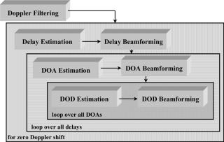
Figure 3.12 illustrates these steps.

The procedure gives us the number and parameters of the MPCs, i.e. the number and values of delays, which DOA can be observed at these delays and which DOD corresponds to each DOA at a specific delay. Furthermore, we also obtain the powers of the multipath channels (MPCs). One important point in the application of the sequential estimation procedure is the sequence in which the evaluation is performed. Roughly speaking, the number of MPCs that can be estimated is the number of samples we have at our disposal.

Figure 3.12 Sequential estimation of the parametric channel response in the different domains: alternating estimation and beamforming. (Reproduced by permission of IEEE [52].)