Advanced Wireless Networks - 4G Technologies

98 CHANNEL MODELING FOR 4G

and transmission characteristics of interior structures of office building in the 60-GHz band,” IEEE Trans. Antennas Propagat., vol. 45, 1997, pp. 1783–1792.

[77]B. Langen, G. Lober and W. Herzig, Reflection and transmission behavior of building materials at 60 GHz, in Proc. IEEE PIMRC’94, The Hague, September 1994, pp. 505– 509.

[78]J.P. Rossi, J.P. Barbot and A.J. Levy, Theory and measurement of the angle of arrival and time delay of UHF radiowave using a ring array, IEEE Trans. Antennas Propagat., vol. 45, 1997, pp. 876–884.

[79]Y.L.C. de Jong and M.H.A.J. Herben, High-resolution angle-of-arrival measurement of the mobile radio channel, IEEE Trans. Antennas Propagat., vol. 47, 1999, pp. 1677–1687.

[80]H. Droste and G. Kadel, Measurement and analysis of wideband indoor propagation characteristics at 17 GHz and 60 GHz, in Proc. IEE Antennas Propagation, Conf. (publication no. 407), April 1995, pp. 288–291.

[81]C.L. Holloway, P.L. Perini, R.R. Delyzer and K.C. Allen, Analysis of composite walls and their effects on short-path propagation modeling, IEEE Trans. Vehicle Technol., vol. 46, 1997, pp. 730–738.

[82]W. Honcharenko and H. Bertoni, Transmission and reflection characteristics at concrete block walls in the UHF bands proposed for future PCS, IEEE Trans. Antennas Propagat., vol. 42, 1994, pp. 232–239.

[83]P. Smulders and L. Correia, Characterization of propagation in 60 GHz radio channels,

Electron. Commun. Eng. J., 1997, pp. 73–80.

[84]H. Xu, T. S. Rappaport, R. J. Boyle and J. Schaffner, Measurements and modeling for 38-GHz point-to-multipoint radiowave propagation, IEEE J. Select. Areas Commun., vol. 18, 2000, pp. 310–321.

[85]H. Xu, V. Kukshya and T. Rappaport, Spatial and temporal characterization of 60 GHz channels, in Proc. IEEE VTC’2000, Boston, MA, vol. 1, 24–28 September, 2000,

pp.6–13.

[86]D. Cassioli, M.Z. Win and A.F. Molisch, The ultra-wide bandwidth indoor channel: from statistical model to simulations, IEEE J. Selected Areas Commun., vol. 20, no. 6, 2002, pp.1247–1257.

[87]L.J. Greenstein, V. Erceg, Y. S. Yeh and M. V. Clark, A new path-gain/delay-spread propagation model for digital cellular channels, IEEE Trans. Vehicle Technol., vol. 46, 1997, pp. 477–485.

[88]V. Erceg, L.J. Greenstein, S.Y. Tjandra, S.R. Parkoff, A. Gupta, B. Kulic, A. A. Julius and R. Bianchi, An empirically based path loss model for wireless channels in suburban environments, IEEE J. Select. Areas Commun., vol. 17, 1999, pp. 1205– 1211.

[89]E. Failli, ed., Digital Land Mobile Radio. Final Report of COST 207. Commission of the European Union: Luxemburg 1989.

[90]M. Nakagami, The m-distribution – a general formula of intensity distribution of rapid fading, in Statistical Methods in Radio Wave Propagation, W. C. Hoffman, ed. Pergamon: Oxford, 1960, pp. 3–36.

[91]W.R. Braun and U. Dersch, A physical mobile radio channel model, IEEE Trans. Vehicle. Technol., vol. 40, 1991, pp. 472–482.

[92]H. Hashemi, The indoor radio propagation channel, Proc. IEEE, vol. 81, 1993,

pp.943–968.

REFERENCES 99

[93]J.C. Liberti and T.S. Rappaport, Smart Antennas for Wireless Communications: IS95 and Third Generation CDMA Applications. Prentice-Hall: Englewood Cliffs, NJ, 1999.

[94]A.A.M. Saleh and R.A. Valenzuela, A statistical model for indoor multipath propagation, IEEE J. Select. Areas Commun., vol. 5, 1987, pp. 128–137.

[95]Q. Spencer, M. Rice, B. Jeffs and M. Jensen, A statistical model for the angle-of- arrival in indoor multipath propagation, in Proc. IEEE Vehicle Technol. Conf., 1997, pp. 1415–1419.

[96]Q. Spencer, B. Jeffs, M. Jensen and A. Swindlehurst, Modeling the statistical time and angle of arrival characteristics of an indoor multipath channel, IEEE J. Select. Areas Commun., vol. 18, 2000, pp. 347–360.

[97]R.J.-M. Cramer, R.A. Scholtz and M.Z. Win, Evaluation of an ultra-wide-band propagation channel, IEEE Trans. Antennas Propagat., vol. 50, no. 5, 2002, pp. 561–570.

[98]S.M. Yano, Investigating the ultra-wideband indoor wireless channel, IEEE 55th Vehicular Technology Conf., VTC, vol. 3, 6–9 May 2002, pp. 1200–1204.

[99]D. Cassioli, M.Z. Win and M.F. Molisch, A statistical model for the UWB indoor channel, IEEE VTC, vol. 2, 2001, pp. 1159–1163.

[100]S.S. Ghassemzadeh, R. Jana, C.W. Rice, W. Turin and V. Tarokh, A statistical path loss model for in-home UWB channels, 2002 IEEE Conf. Ultra Wideband Systems and Technologies, Digest of Papers, 21–23 May 2002, pp. 59–64.

[101]W. Turin, R. Jana, S.S. Ghassemzadeh, C.W. Rice and T. Tarokh, Autoregressive modelling of an indoor UWB channel, IEEE Conference on Ultra Wideband Systems and Technologies, Digest of Papers, 21–23 May 2002, pp. 71–74.

[102]S.S. Ghassemzadeh and V. Tarokh, UWB path loss characterization in residential environments, IEEE Radio Frequency Integrated Circuits (RFIC) Symp., 8–10 June 2003, pp. 501–504.

[103]S.S. Ghassemzadeh and V. Tarokh UWB path loss characterization in residential environments, IEEE MTT-S International Microwave Symposium Digest, vol. 1, 8–13 June 2003, pp. 365–368.

[104]G.H. Golub and C.F. Van Loan, Matrix Computations, 3rd edn. The Johns Hopkins University Press: Baltimore, MD, 1996.

[105]P. Petrus, J.H. Reed and T.S. Rappaport, Effects of directional antennas at the base station on the Doppler spectrum, IEEE Commun. Lett., vol. 1, 1997, pp. 40–42.

[106]W.C.Y. Lee, Estimate of local average power of a mobile radio signal, IEEE Trans. Vehicle Technol., vol. 34, 1985, pp. 22–27.

[107]E. Green, Radio link design for micro-cellular systems, Br. Telecom. Technol. J., vol. 8, 1990, pp. 85–96.

[108]U. Dersch and E. Zollinger, Physical characteristics of urban micro-cellular propagation, IEEE Trans. Antennas Propagat., vol. 42, 1994, pp. 1528–1539.

[109]Y. Karasawa and H. Ivai, Formulation of spatial correlation statistic in Nakagami-Rice fading environments, IEEE Trans. Antennas Propagat., vol. 48, 2000, pp. 12–18.

4

Adaptive and Reconfigurable

Link Layer

4.1 LINK LAYER CAPACITY OF ADAPTIVE AIR INTERFACES

In wireless systems, the channel reliability is affected by several phenomena, such as the propagation properties of the environment and mobility of terminals. To compensate for these impairments, various techniques are used at the physical layer, including adaptive schemes, which dynamically modify the transceiver structure. As a consequence of varying channel conditions and dynamically changing transceivers structures, the available information data rate at the link layer is in general time-varying. The channel seen from above the physical and link control layer, which will be referred to as a medium access control (MAC) channel, must be characterized with sufficient accuracy but still by a simple model that can be used in the analysis of the higher network layers. In the resulting MAC channel model used in this chapter, physical layer characteristics, as well as the physical channel and some implementation losses, are taken into account. The efficiency of the model is improved, avoiding bit level or signal level and detailed channel statistics calculations. The result is a model that can be easily used for analytical purposes, as well as for efficient modeling of the MAC channel behavior in network simulators. Owing to its modular structure, the analysis can be extended to more general and possibly complicated systems. In general, the physical layer, or layer 1 (L1), provides a virtual link of unreliable bits. For the sake of simplicity, in this chapter we will use the term physical layer (PHY) when referring to the protocol stack portions in which no distinction is made regarding the information carried by the bits. The portions in which such a distinction is made will be referred to as upper layers. This corresponds to L2–L7 of the International Standardization Organization–Open System of Interconnections (ISO-OSI) model.

The model discussed in this chapter includes a physical channel and the physical layer (Figure 4.1) [1]. The same portion of the protocol stack is covered in a link layer model,

Advanced Wireless Networks: 4G Technologies Savo G. Glisic

C 2006 John Wiley & Sons, Ltd.

102 ADAPTIVE AND RECONFIGURABLE LINK LAYER

PHY

Adaptive TRX

r0	r1	r2	r3		rM-1
e0	e1	e2	e3	λ3	eM-1
	λ 0	λ1	λ2		λM-2
0	1	2	3	...	M-1
	μ1	μ2	μ3	μ4	μM-1

CH

Figure 4.1 The MAC channel model that includes the overall behavior of the physical channel and the PHY. According to the channel state, the PHY mode is chosen. As a consequence, in each state, data rate ri and error rate ei are defined. The model includes imperfections in the implementation of the adaptation method.

called the effective capacity link model [2], which models directly some link layer parameters used in queuing analysis without including imperfections of the physical layer or adaptation in the link layer. A similar definition of MAC channel is given in Liebl et al. [3], where a model for packet losses is included, taking into account physical channel, modulation and channel coding, and some other functions of the data link layer, but only for transceivers with fixed structure.

In order to extend Gilbert [4], Gilbert–Elliot [5], Fritchman [6] or bipartite models [7], as hidden Markovian models [8], to a finer granularity of error rates or larger dynamic range with adaptation techniques at the physical layer, finite-state Markov chains with larger numbers of states have been introduced, e.g. in Wang and Moayeri [9]. The basic approach is to quantize the signal envelope or the range of the signal to interference-plus- noise ratio (SINR), and associate each state of the Markov chain with a given range, to model the packet error process in the presence of a fading channel. In Steffan [10], the error process is modeled as the ‘arrival’ of errors, with arrival rate varying according to a Markov-modulated process (MMP). In the existing literature, the Markov model is often considered for Ricean or Rayleigh fading channels. It has also been applied to other statistical models, such as Nakagami fading channels [11], or built from error traces obtained from measurements [12]. The validity of the first-order Markov model is addressed in References [13–18]. The accuracy of the model can be assessed by using information theoretic [15] or probabilistic approaches [18]. In Babich and Lombardi [18], it is reported that the first-order Markovian model, in which the states represent discrete, non-overlapping intervals of the signal envelope’s amplitude, is not suitable to model very slow fading channels unless the analysis is carried out over a short time duration. However, it is also pointed out that this applies to bit-level systems, whereas the model can be valid for block-level systems. The performance of adaptive radio links has been studied in presence of an AWGN channel [19], or fading channels but without channel coding [20], or for coded systems analyzed under specific channel coding schemes and decoding methods [21, 22].

LINK LAYER CAPACITY OF ADAPTIVE AIR INTERFACES

103

The goal of this chapter is not to capture effects of higher frequency fading, but rather to represent the behavior of the signal quality level in terms of presence in a region, and to link it to the behavior of the service offered by the PHY in terms of data rate and error rate, with a granularity given by the number of PHY modes of the system. When the number of regions is small, e.g. less than eight, the quality level exhibits lower frequencies owing to practical constraints discussed in the following sections. In this chapter, a continuous, rather than discrete, time channel model is used. The benefit of this approach is 3-fold. First, the model may be integrated better in some broader analytical models, and the simulation model that can be derived from it can be efficiently integrated in event-driven simulators, which are usually more efficient. Second, the model presented in this chapter integrates both channel model and link adaptation in a flexible way open to generalizations. Third, some imperfections such as channel estimation error, estimation delay and feedback error, as well as implementation implications, like switching hysteresis, are included in the model.

4.1.1 The MAC channel model

We are interested in modeling the properties of the service capacity offered by the PHY to the upper layers, rather than in the rigorous characterization of the physical channel. The service capacity is basically given by the gross transmission bit rate and the errors at the receiver. In absence of link adaptation, i.e. with one fixed PHY mode, the gross bit rate is constant across channel states and the error rate absorbs the variability of the channel. Conversely, with link adaptation, the error rate is kept bounded whereas the bit rate changes with the state of the channel. Our model captures the dynamics of those metrics by modeling the channel as seen from above the PHY (Figure 4.1). The model therefore includes the physical channel and the PHY characteristics. In this chapter this model is referred to as the MAC channel. The MAC channel is modeled as a finite Markov chain (Figure 4.1), in which each state corresponds to a PHY mode and is hence associated with a specific transceiver configuration. In an adaptive modulation and coding (AMC) system, a mode corresponds to a modulation and channel coding schemes pair, and hence to the transmit bit rate and the error rate. The link service capacity characterized in this chapter, denoted Rc(t) and defined later, is actually a stochastic process Rc(t; ζ ), which depends on the PHY mode in use, which is selected depending on the signal quality level estimate γˆ (t; ζ ). In the notation to follow, unless otherwise specified, the dependence on time t and realization ζ will be omitted.

4.1.2 The Markovian model

Packets or symbol channel errors may be observed at sampling instants using a model time unit equal to packet or symbol interval. This approach is often used for error models at both symbol and packet level error analysis [9, 23]. In this case, if a Markovian model is adopted, the resulting model is discrete time.

Channel conditions may be represented by the value of some metric of the link quality γ , whose domain is divided in non-overlapping regions. In the model considered in this chapter, changes in the state of the system coincide with boundary crossings of this metric. We model the true quality level as a continuous-time Markov chain with the state of the

104 ADAPTIVE AND RECONFIGURABLE LINK LAYER

model representing the signal quality region. Typical fading channels exhibit correlation between successive values and therefore the system cannot be considered as memory-less if samples of those values are analyzed. However, in our system the process state is represented by the γ -region which corresponds to a PHY mode. This correspondence has been outlined above and will be described in detail in the following section. The number of PHY modes is typically small. For example, the high-speed downlink packet access (HSDPA) of the UMTS terrestrial radio access (UTRA) envisages seven modes, whereas IEEE 802.11a and the ETSI HIPERLAN/2 have seven and eight modes, respectively.

In continuous time model, the system does not sample the specific value of the quality metric, but rather the region in which the quality metric falls. It is clear that for a small number of states the higher frequency correlation in the physical channel is smoothed out when considering the jumps from one state to another. The assessment of the validity of the Markov property assumption may be feasible for simple statistical physical channel models, but may be impossible with more complicated channel models or for models derived from measurements. The framework presented in this chapter is intended to be applicable to generic channel processes that are continuous, based on known statistics or on heuristics, and that can be represented by a small number of states. The true channel quality level is modeled as a continuous time Markov chain (CTMC).

Let us consider a continuous-time finite Markov chain obtained by a stochastic process γ (t; ζ ) defined over a time interval T (−∞, +∞) which assumes values on a continuous set R split in a finite number of contiguous, nonoverlapping intervals. If the process is continuous, then the CTMC is a birth–death process, since the new value assumed by a continuous function after an infinitesimal time interval t can only belong to the same or a neighboring interval. For our purpose, it is sufficient to assume that the process is continuous. So, looking at the time instants in which γ crosses the target levels, the process can jump only to neighboring states.

We now define the elements of the state transition rate matrix, Q, also known as infinitesimal generator or intensity matrix. With state Si associated with γ [γi , γi+1), see Equation (4.3), the generic elements of Q can be written as

q

k,k+1

=

p(k, k + 1; t, t + t)

=

Pr{crossing upwards in t|Sk }

t

Nk++1

t

=

Nk++1 t 1

=

(4.1)

πk t

πk

where Nk+ is the expected number of times level k is crossed upwards in a second (the level crossing rate, LCR), and πk is the probability of state Sk . Going from Sk to Sk+1 is defined by crossing the threshold γk+1. Similarly,

			p(k, k	−	1; t, t	+	t)		N −
q	k,k−1	=						=	k	(4.2)
					t				πk

For practical reasons described later, a certain hysteresis at switching points is introduced. In this case, the definition of LCRs Nk++1 and Nk− is modified by considering the levels γk+1 + ϕk++1 and γk − ϕk−, respectively. The interpretation of the term πk with hysteresis is discussed later. Note that, by rewriting Equation (4.1) as p(k, k + 1; t, t + t) = qk,k+1 t + o( t), replacing t = Tu , where Tu is the time unit of a discrete time model, we obtain the expression of the transition probability of the discrete time Markov chain representing

LINK LAYER CAPACITY OF ADAPTIVE AIR INTERFACES

105

symbol or packet errors, used (without the concept of hysteresis) in Brummer¨ [8] and related papers [12].

The quantities in Equations (4.1) and (4.2), namely the level crossing rate and state probabilities, are found in literature for some common processes like Rice and Nakagami. For more complicated channel models or for measurements traces when the terms in the right-hand sides of Equations (4.1) and (4.2) are not known, those quantities can be easily evaluated from the observation of the measurement traces or from link-level simulations of the possibly complicated models, by observing that the LCRs and state probabilities are Nk± ≈ n±k /t and πk ≈ tk /t. In these expressions, n+k and n−k are the number of crossing levels γk upwards and downwards, respectively, tk is the time spent in region Sk , and t is the total observation time. By replacing these expressions in Equations (4.1) and (4.2), we obtain qk,k+1 = n+k+1/tk and qk,k−1 = n−k /tk .

4.1.3 Goodput and link adaptation

The received signal quality can be measured, for example with the SINR, but in the following we will denote with γ a generic metric for the quality level. The signal quality is a function of a number of contributions, related to both the transceiver structure and settings and the communication environment. Changes in the time-varying signal quality are due to various factors which change with different speed. Changes occurring in periods comparable with bit rate duration, O(Tbit), or shorter, are dealt with typically with diversity gain. Slower changes, occurring in periods comparable with packet interval, O(Tpkt), are handled by changing PHY schemes and possibly by proper scheduling. Changes of O(Tframe) and greater are handled typically with scheduling or renegotiations and reconfigurations at higher layers. In addition to diversity gain and multiplexing gain [24], link adaptation techniques are used to enhance performance. As a response to the received signal quality γ , link adaptation algorithms initiate changes in the transceiver structure Kr , keeping a performance metric e between certain boundaries: e(Kr , γ ) {acceptable values}. Link adaptation strategies include changing both modulation and channel coding schemes (referred to in the literature as adaptive modulation and coding), and transmission power, or the combinations of the two [25]. A larger number of transceiver configuration parameters can be adaptively adjusted according to some strategy. This leads to the concept of PHY mode, extension of the AMC and in line with the idea of software-defined radio (SDR).

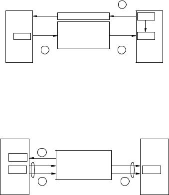
The definition of the reference and control signals that are fed into the adaptation algorithm is the basis of adaptive systems. These are the target quality and the actual signal quality, respectively. Basically, there are two possible methods for the definition of the control signal. The first is to let the transmitter know what the measured quality at the receiver is (Figure 4.2). Being a closed loop solution, it has the drawbacks that the signal that is used by the algorithm does not reflect the channel conditions at the transmission time, and that the control message itself is subject to errors in the feedback channel. The other possibility is that the transmitter autonomously estimates the channel, based on the quality measured at its own side (Figure 4.3). This open loop scheme assumes reciprocity of the direct and feedback channels. UMTS TDD is an example of the system where such approach is possible. In both cases, a related problem is how transmitter and receiver agree their configuration. With closed loop, the channel status information is sent from the receiver to the transmitter, e.g. by piggybacking the information on outgoing packets. In this

106 ADAPTIVE AND RECONFIGURABLE LINK LAYER

	1
	EST
c(t) CONFIG	CONFIG
	CH
2	3
TX	RX

Figure 4.2 Adaptive radio with receiver-controlled link adaptation, or closed loop control of mode switching. The receiver does the channel estimation and communicates the channel quality or directly commands the transmitter the mode to be used. Numbers indicate the sequence order of operations. Solid lines are data transmission, whereas dashed lines are control signaling. The metric used as a control signal, c(t) ≈ γˆ (t − τe), is a delayed estimate of the true channel quality value, possibly affected by errors in the feedback channel.

1
EST
c(t) CONFIG	CONFIG
	CH
2	3
TX	RX

Figure 4.3 Adaptive radio with transmitter-controlled link adaptation, or open loop control of mode switching. The transmitter first estimates the state of the channel based on the received signal, and then transmits data. Some coded information about the chosen mode must be sent, or complexity at the receiver must be added to estimate the mode. Numbers indicate the sequence order of operations. Solid lines are data transmission, whereas dashed lines are control signaling. The metric used as control signal, c(t) = γ˜ (t), is an approximated estimate of the true channel quality value. The value is also affected by the lack of channel reciprocity in two directions.

receiver-controlled scheme the PHY mode will be obviously known at the receiver side. Conversely, in the open loop case, the mode can be either sent by the transmitter, causing overhead, or obtained blindly from the receiver, leading possibly to an increase in complexity and to PHY mode acquisition errors. It must be emphasized that, with both open and closed loop schemes, it is practically impossible for the transmitter to know what the actual channel state will be at the transmission instant at the receiver. Imperfections in the adaptation chain have an impact on the effectiveness of the algorithm. Indeed, the closed loop scheme is affected by delay, which is not less than the round trip propagation delay, and possibly by channel state estimation error. The open loop is affected by a much smaller estimation delay, but the estimate may not match the state at reception site and time. In addition to that, the information signaled from the receiver to the transmitter is prone to

LINK LAYER CAPACITY OF ADAPTIVE AIR INTERFACES

107

errors in the communication channel. All these aspects are taken into account in the model for imperfections described in the next section.

The error rate is a fundamental performance measure for QoS for both delay-insensitive and delay-sensitive services. According to QoS requirements, certain target error rates can be identified, and from them, the domain of the signal quality metric can be divided into M, nonoverlapping intervals. Each region is associated with a state of the CTMC S = {S0, S1, . . . , SM−1}. According to the adaptation algorithm, one of the M PHY modes (a modulation and channel coding scheme pair) available in the system is associated with each region of the signal quality metric: M = {M0, M1, . . . , MM−1}. Each state is therefore

characterized by the bit rate and the error rate: Si Mi ri ,	ei . The set of the threshold
levels, the mode switching points, {γi }, i = {0, . . . , M}, is defined so that:
γ [γi , γi+1) Si Mi , 0 < i ≤ M − 1
γ (γ0, γ1) S0 M0	(4.3)

where γ0 = −∞ and γM = +∞. For the PHY mode Mi the selection must comply with the requirement ei ≤ emax, 0 ≤ i < M, where emax is the maximum tolerable error rate, i.e. the target error rate. By noting that e(γ ) is a monotonic decreasing function of γ , we have γi = e−1(emax). If the statistics of the channel process are known, the nominal value of the signal quality metric in each region can be defined as follows:

	γi+1	γi+1
γ¯i =	γ pγ (γ ) dγ	pγ (γ ) dγ	(4.4)
	γi	γi

If not, it can be simply represented by the center value in the range.

Switching points can be determined also using methods other than the one described above, including optimization [26]. The model described in this chapter is independent of the method used.

4.1.4 Switching hysteresis

As with all real control systems, if the same threshold value was chosen for both process rising and falling thresholds, the system could exhibit too frequent mode switching. A solution to this known problem is to introduce a hysteresis, fixing two distinct values for falling and rising thresholds. If γ − and γ + are falling and rising threshold values, respectively, the actual threshold values will be defined as:

γi± = γi ± ϕi±

(4.5)

With ϕi+ = ϕi− = ϕi = ϕ, 2ϕ is the width of the hysteresis region. Another choice is to select the switching thresholds k accordingly to the following equation:

γk	γk +ϕk+
pγ (γ ) dγ =	pγ (γ ) dγ	(4.6)
γk −ϕk−	γk

This definition can be applied independently of the method used to define the ideal threshold levels. For example, an effective definition of switching points could be obtained by imposing an upper limit on the probability of spurious switching in a given time.