Cleaver Economics The Basics (Routledge, 2004)

coffee increases, demand for it will fall, and vice versa, assuming all other factors influencing the market remain unchanged.

The slope of the demand curve illustrated is important. It shows just exactly how much demand will contract as price increases a little or, conversely, how much demand extends as price falls.

The slope of the demand curve thus helps to represent the responsiveness, or ELASTICITY, of demand consequent to a change in price. All things being equal, the flatter the demand curve the more responsive or price-elastic is demand. Figure 2.7 shows a situation where a small change in price is met by a large change in the quantity demanded (Box 2.3).

Price

Price-elastic

demand

Quantity

0

Figure 2.7 Price-elastic demand.

Box 2.3 Calculating price-elasticity

Actually, since the flatness or steepness of any curve illustrated depends entirely on how scale is represented on the vertical axis, it is best to refer to the elasticity of demand mathematically. If a 5 per cent fall in price is met by a 20 per cent extension in demand then we can say that demand is very price-elastic. Elasticity is measured as the ratio of the percentage change in quantity to the percentage change in price – in this case equal to 20/5 or equal to 4.

© 2004 Tony Cleaver

Conversely, a steep demand curve illustrates ceteris paribus a less responsive or inelastic relationship to a price change (Box 2.4).

Box 2.4 Price-inelastic demand

You should be able to see that whereas goods and services that are price sensitive have a ratio of price-elasticity greater than 1, goods for which there are no or few substitutes will have a priceelasticity of less than 1. For example a 400 per cent increase in the world price of oil in January 1974 let to a minimal reduction (say 6 per cent) in demand. That gives a ratio of 6/400 or 0.015!

Generally speaking, the more one good can be substituted for another in your pattern of spending, the more price-elastic it is likely to be in demand. If Shell petrol goes up in price, for example, and no other prices change then most consumers will simply switch to alternatives such as BP or Esso. Demand for Shell oil is highly price-elastic. If all oil goes up in price, however, then consumers have no substitute for this vital commodity and market demand may not change much at all in the short run. Demand for all oil is price-inelastic.

S h i f t s i n D e m a n d

The analysis in the previous section has referred to price movements, ‘all other factors remaining unchanged’. But what factors other than price have an important influence on market demand and how do they affect the theory being developed here?

For any one commodity, a whole range of other factors can be listed. World demand for coffee, for example, is affected by changes in consumers’ incomes, by industry advertising, by collective fashions, tastes and preferences, by competition from alternatives or complementary goods, perhaps even by global changes in the climate. Whatever the price of coffee, if any of these other factors changes it will cause – to a great or lesser extent – a shift in demand.

Suppose, for example, the International Coffee Organisation sponsored a successful, world-wide advertising campaign to promote the consumption of coffee. Then, whatever the going

© 2004 Tony Cleaver

market price, we can expect that many more consumers would enter the market and buy coffee. In Figure 2.8 at price P1, for example, demand shifts from quantity Q1 to Q2.

Demand for coffee can change for any number of reasons, therefore. A contraction (or extension) in demand caused by an increase (or decrease) in price is illustrated by a movement along the demand curve. A fall (or rise) in demand caused by any other exogenous change is illustrated by a shift in the whole curve (Boxes 2.5 and 2.6).

Price

P1

D2

D1

Quantity

0Q1 Q2

Figure 2.8 A demand shift.

Box 2.5 Endogenous and exogenous changes

A two-dimensional diagram can only illustrate the interactions between two variables – in this case, the effect of price on demand. In this particular example, an increase in price is an endogenous change, that is to say within the dimensions of the model, and its effect can be studied on the dependent variable: causing a fall in demand illustrated by a contraction along the demand curve. A change in some other factor outside the model, in this example advertising, is an exogenous change and this causes the relationships between the two original variables to shift. The distinction between endogenous (internal) and exogenous (external) changes is important and will be referred to continually through this text.

© 2004 Tony Cleaver

Box 2.6 Coffee prices: part 1

All this analysis may seem a bit pedantic but, as you will see later on, it is actually important in separating out causes and effects of major crises in world markets. A quick example should help explain. Coffee is (after oil) the world’s second most important traded commodity. The livelihood of 25 million small producers and more than half-a-billion other people linked to the coffee trade in poor countries is directly influenced by the price of coffee. At the time of writing, the world price of coffee is close to a 100-year low – depressing the incomes, and lives, of millions. Additionally, prices over the last twenty years have been very volatile – hurting particularly the smaller farmer who cannot insure against risk.

Is the price low because world demand is low or has some other factor caused the slump in prices? And what causes the sudden and great reversals in prices and fortunes? This is not an insignificant matter. Careful analysis is called for . . .

200
150
100
50
0
Oct-83	Oct-86	Oct-89	Oct-92	Oct-95	Oct-98

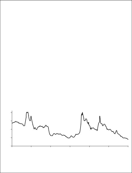
Figure 2.9 Coffee Prices, 1983–2002.

Source: ‘Coffee Market Trends’ Kristina Sorby, World Bank (June 2002).

M a r k e t S u p p l y

The incentive for any business to supply goods to market is to make profits – to sell his/her product at a higher price than the COSTS OF PRODUCTION involved in offering it for sale. Whether it be a personal service, such as providing haircuts, the assembly of a luxury motor

© 2004 Tony Cleaver

car with inputs from all over the world, or selling advertising space on-line to invisible consumers, these goods and services will only be supplied if the market price agreed on with the buyer sufficiently rewards the entrepreneur for his/her efforts.

Assume that all suppliers wish to maximise profits. Given that production costs and all other factors affecting the supply of a certain good remain constant, then producers will increase supplies to the market if prices rise. Conversely, supply will contract if price falls.

There are many costs involved in offering coffee for sale in a given market place. At low prices per cup, only the most efficient, low-cost suppliers can afford to produce this beverage and the quantities offered for sale will be limited. If consumers are willing to pay higher prices, however, then other suppliers will be tempted to enter the market and existing producers will also increase their provision. At very high prices, businesses which had never previously thought of making this product may well switch production plans and become coffee suppliers.

We can illustrate the relationship between the price of a product and the quantity supplied by the supply curve S in Figure 2.10.

Note that, as before, the slope of the supply curve indicates the responsiveness of producers to alter supplies as price changes. If, for example, a small increase in price calls forth a proportionally large increase in quantity then supply is said to be price-elastic. The rather steep curve shown here illustrates the opposite: relatively low price-elasticity of supply.

Price-elasticity of supply is affected by time – the longer businesses have to adjust production plans, the more responsive they

S

Price

Quantity

Figure 2.10 A supply curve.

© 2004 Tony Cleaver

(a)	(b)	(c)
Price	Fixed	Price-inelastic	Price-elastic supply
	supply	supply

Quantities

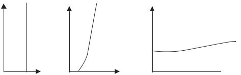
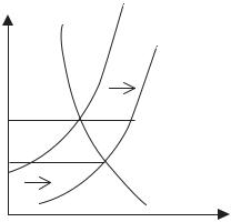
Figure 2.11 Changes in price-elasticity of supply over time. (a) Spot market,

(b) the short term and (c) the long term.

can be to any market changes. A sudden increase in demand for almost any product cannot be accommodated instantly, no matter how high a price a customer is prepared to pay. Supplies of oil, cars or coffee, for example are fixed by current stockpiles. If someone is desperate to buy something then a high price may persuade another consumer to leave the market (as in an auction) but supply itself cannot be increased.

Over time, depending on the technology involved in production, high prices call forth greater supplies. For oil, more may be pumped out of the existing wells and refineries. More cars can roll off the assembly line. In the case of coffee, if all existing stocks are already committed, consumers will have to wait until the next harvest.

Typically, economists can identify three trading periods: the instantaneous or SPOT MARKET, when supplies are fixed to existing, identifiable stocks; the SHORT TERM when supplies are price-inelastic and the LONG TERM when supplies are price-elastic (Figure 2.11).

The dividing line between the short term and long term is a matter of judgement. The short term usually refers to the increase in supplies that can be gained by relying on existing resources and working them harder; the longer term tends to imply employing more factors of production.

S h i f t s i n S u p p l y

What other factors than price affect supplies? A supply curve for any good or service shows the distinctive relationship between just one variable, price and the quantity of supplies that each price will call forth to the market. As before, if any exogenous variable

© 2004 Tony Cleaver

	Price of beer		Supply after tax
	(per pint)			Supply curve of beer
	P1 + £x		£x
	P1
	0			Quantity
		Q2	Q1

Figure 2.12 A shift in supply.

outside of this relationship changes then the original supply curve will shift in its entirety – showing that at whatever price that existed before, now at that same price a new supply relationship exists.

Any sudden change in production costs, say due to a technological breakthrough or breakdown, an increase in wages, any transport and distribution hold-up, will all effect a shift in supply (Figure 2.12). Government tax and regulation can also affect supplies of certain goods and services.

If a local brewery was prepared to supply quantity Q1 of beer to town at a price of P1 and then the government raises the beer tax by £x per pint sold then this will shift the supply curve as shown. That is, the brewery will only be prepared to sell the same quantity as before at a price of P1 £x. Equally, if they had to pay the tax at the old price P1 then the brewery would only be prepared to supply the much-reduced quantity Q2.

P R I C E D E T E R M I N AT I O N : A C A S E S T U D Y

We now have all the analytical components in place to complete our theory of price. To recap, price changes signal how resources in the economy must automatically re-allocate so as to match consumer demand to potential supplies. How does this work? How are sudden changes in market preferences or in production conditions accommodated in an economy and what are the implications for the people involved?

Consider again the world market for coffee, which is the most important agricultural commodity that is traded internationally and

© 2004 Tony Cleaver

is currently exported from fifty-two countries. Since the mid-1990s, world production of coffee has dramatically increased, mainly due to continued expansion in Brazil and the recent entry of Vietnam as a major producer with its new plantations now bearing fruit. (Coffee production in Vietnam has increased 1400 per cent between 1990 and 2000!) Other big producers of coffee, such as Colombia, have maintained stable or slightly falling supplies over the same period.

Global demand for coffee has not shown an increase on the same scale as supply over the last few years. There is a change in consumer tastes within the coffee market – in favour of more organic, environmentally friendly products – but overall consumption has increased hardly at all, relative to supply.

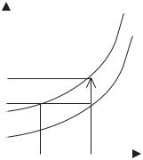
We can illustrate this in Figure 2.13 as follows. World demand for coffee is stable and relatively price-inelastic as illustrated by the demand curve shown. World supply is also relatively price-inelastic and is illustrated by supply curve S1. Supply, however, is unstable in that Vietnam’s drive to increase exports and incomes at home has meant increased efforts to plant and produce coffee. The supply curve therefore shifts to S2, there being no reduction in supplies elsewhere in the world.

At the old price P1, the world demand for coffee is represented by the distance P1A. World supply is now greater and equals P1B. With an excess supply of AB in world markets, the price will be under pressure to fall. As it does so this induces some extension in demand (an increase in quantity illustrated by movement along the demand curve from A to C) and simultaneously some contraction in supply (movement from B to C). In time, a new market equilibrium will

Price	Demand	S1
		S2
P1	A	B
P2		C

0	Quantity

Figure 2.13 Prices in the world coffee market.

© 2004 Tony Cleaver

evolve at C at a lower price P2 and a small increase in the quantity of coffee traded, equal to P2C.

Note that so long as the demand curve is stable and priceinelastic (relatively steep) then relatively small shifts in supply (due to sudden increases or decreases in coffee harvests) will cause relatively large changes in price, as shown earlier. The irony is that for small producers who are anxious to increase outputs and increase their incomes, if they are collectively successful then the result of their efforts is to drive coffee prices down a long way – thus significantly reducing their incomes! Individual farmers may not increase production so much themselves, but they are dependent on world markets and as prices fall, they and their family will face increased hardship, if not actual poverty.

In this example, the chain of events has been as follows: a change in the factors affecting production (sudden entry of a new, large producer) has caused excess supplies, which has pushed down the world market price and this has called forth just enough increased demand to buy up the excess.

The truth is that almost all agricultural markets are vulnerable to sudden fluctuation brought about by exogenous shocks. Good harvests can produce bumper crops one year, which push prices down, or another year natural disasters can decimate production, causing prices to soar. Farmers have uncertain incomes, therefore, and the ill fortune which visits one family and destroys their crop may push up prices and reward another lucky enough to escape and bring their supplies to market (see Box 2.7).

Sudden shocks in supply conditions are common in agriculture. In contrast, movements in consumer demand tend to be less frequent and more long-drawn-out since peoples’ consumption habits are typically slow to change. The final example for this chapter looks at the effects of one such development in demand – the environmental movement.

Although it has been mentioned that aggregate world demand for coffee has been stable over recent years, there has nonetheless been a swing within the market towards purchasing the product of more sustainable agricultural practices. The World Bank estimates that demand for certified organic coffee is currently increasing at around 15–18 per cent per year. Such a demand is delivering a considerable price premium to the farmers involved.

© 2004 Tony Cleaver

Box 2.7 Coffee prices: part 2

In reality, all sorts of factors change all the time so that prices are constantly on the move. In 1997 a severe drought in Brazil destroyed a large fraction of the coffee harvest which caused a sudden peak in world prices (see Figure 2.9). Since then however supplies have steadily increased and prices fallen to an all-time low, as already explained. The International Coffee Organisation report that world production in the crop year 2001/02 totalled 109.8 million bags, rising to 120 million bags in 2002/03. This data compares to a relatively stable demand, estimated at 108.3 million bags in 2002. No wonder that prices slumped!

Predictions for the future, however, indicate cutbacks in production. This is so particularly in Brazil for the following reasons: First, there is a biennial production cycle which means that very good harvests are normally followed by poor ones. Second, recent low prices, earnings and profits in the plantations have meant maintenance difficulties which inevitably depletes future production potential. Last, there has been a recurrence of drought. Add to this contractions in production predicted for other countries where agricultural costs have also risen whilst coffee revenues have fallen and the outlook for world prices looks uppish. The forward shifts in supply illustrated earlier which have caused prices to fall should be followed by shifts back in supply to return the market to close to where it was before. Farmers are hoping for higher earnings.

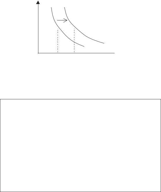
Consider the supply conditions for traditional, smallholder coffee, grown on mountain slopes at the interface between primary tropical rainforest and cleared agricultural land. Such coffee naturally grows in the shade of a forest canopy that supports a rich flora and fauna and is not uncommon for many small farms in Central America. Some investment will be required to have this traditional practice certified as ‘organic’ or ‘shade-grown’ but the benefit for the smallholder of such certification can be illustrated as seen in Figure 2.14.

© 2004 Tony Cleaver