

Bologna / 04_TCAD_laboratory_pn_junction_GBB_20150223H1655
.pdfSdevice input file (2)
Physics
{
Mobility ( DopingDependence
)
Recombination (
#if @SRH@ == 1 SRH
#endif
)
AreaFactor=2
}
the device in this example is 2D. By default, the width in the third dimension is taken to be equal to 1μm. By specifying this value, on the contrary, currents are multiplied by AreaFactor, which in this example with take equal to 2 μm
activation of physical models
G. Betti Beneventi 21

Sdevice command file (3)
Plot
{
* On-mesh-defined variables to be saved in the .tdr output file *- Doping Profiles
Doping DonorConcentration AcceptorConcentration *- Charge, field, potential and potential energy
SpaceCharge ElectricField/Vector Potential
BandGap EffectiveBandGap BandGapNarrowing ElectronAffinity
ConductionBandEnergy ValenceBandEnergy |
|
*- Carrier Densities: |
|
EffectiveIntrinsicDensity IntrinsicDensity |
These keywords under the Plot |
eDensity hDensity |
section allow plotting the distributed |
eQuasiFermiEnergy hQuasiFermiEnergy |
quantities simulated (both scalar |
*- Currents and current components: |
and vectors). |
eGradQuasiFermi/Vector hGradQuasiFermi/Vector |
Some of the keywords refer to |
eMobility hMobility eVelocity hVelocity |
quantities that are calculated only if |
Current/Vector eCurrent/Vector hCurrent/Vector |
the respective physical model are |
eDriftVelocity/Vector hDriftVelocity/Vector |
activated. Anyway, the keywords |
*- SRH & interfacial traps |
can be included in the Plot section |
SRHrecombination |
command file even if the respective |
tSRHrecombination |
models have not been activated |
|
(useful to have a standard template |
|
of Plot section) |
|
|
|
G. Betti Beneventi 22 |

Sdevice command file (4)
*- Band2Band Tunneling & II
eBand2BandGeneration hBand2BandGeneration Band2BandGeneration eAvalanche hAvalanche Avalanche
}
Math
{
*use previous two solutions (if any) to extrapolate next Extrapolate
*use full derivatives in Newton method
Derivatives
*control on relative and absolute errors -RelErrControl
*relative error= 10^(-Digits)
Digits=5
*absolute error Error(electron)=1e8 Error(hole)=1e8
*numerical parameter for space-charge regions eDrForceRefDens=1e10
hDrForceRefDens=1e10
*maximum number of iteration at each step Iterations=20
*choosing the solver of the linear system Method=ParDiSo
G. Betti Beneventi 23

Sdevice command file (5)
*display simulation time in 'human' units Wallclock
*display max.error information CNormPrint
*to avoid convergence problem when simulating defect-assisted tunneling NoSRHperPotential
}
Solve
{
* EQUILIBRIUM
coupled {poisson}
MaxStep must be higher than MinStep
*TURN-ON
*decreasing p_contact to goal
quasistationary (InitialStep = 0.010 MaxStep = 0.050 MinStep=0.005 Goal {name= "p_contact" voltage = @V_start@}
plot { range=(0, 1) intervals=1 }
)
{coupled {poisson electron hole} }
Newton iteration
G. Betti Beneventi 24

Sdevice command file (6)
* raising p_contact to goal * negative part
quasistationary (InitialStep = 0.010 MaxStep = 0.050 MinStep=0.005 Goal {name= "p_contact" voltage = 0}
)
{coupled {poisson electron hole} }
quasistationary (InitialStep = 0.010 MaxStep = 0.050 MinStep=0.001 Goal {name= "p_contact" voltage = @V_stop@}
plot { range=(0, 1) intervals=15 }
)
{coupled {poisson electron hole} }
}
•Save Quit
G. Betti Beneventi 25
Sdevice: write the parameter file (1)
•How to get the material parameters for Silicon, Germanium and GaAs and assembly a single parameter file for Sdevice simulation containing all the parameters for physical models:
from the terminal commandline
GO TO PROJECT DIRECTORY cd ~/TCAD/pn_ideale
PRODUCE TEXT FILES WITH PARAMETERS. ONE FOR EACH MATERIAL sdevice –P:Silicon > sdevice.par
sdevice –P:Germanium >> sdevice.par sdevice –P:GaAs >> sdevice.par
OPEN FILES sdevice.par AND CUT THE LOG INFORMATION, that is:
CUT THE HEADERS FOR EACH MATERIAL AND CONSERVE ONLY THE PART STARTING FROM
Material= "Silicon" {
TO LAST }
DO THE SAME FOR EACH MATERIAL (see next slide)
G. Betti Beneventi 26

Sdevice parameter file (2)
•The sdevice.par file should appear like this:
Material = "Silicon" {
Epsilon {
…
}
}
Material = "Germanium" {
Epsilon {
…
}
}
Material = "GaAs" {
Epsilon {
…
}
}
SWB needs at least an empty file. If material parameters must not be
modified compared to the default values, even an empty file will do the job. However, create the parameter files is useful to check which parameters are used for a given material for a given model (and, in case, change their values)
DONE Sdevice PART
G. Betti Beneventi 27

Outline
•Review of basic properties of the diode
•Sentaurus Workbench setup (SWB)
•Implementation of Input files
–Sentaurus Structure Editor (SDE) command file
–Sentaurus Device (SDevice)
•command file
•parameter file
Run the simulation
• Post-processing of results
G. Betti Beneventi 28

Run the simulation
•on SWB interface
PREPROCESS ALL NODES (software writes sde, sdevice and parameters file for each experiment)
CTRL-P
•RUN SDE
Select all real(*) nodes of Sde CTRL-R Run
wait for the real nodes becoming yellow (i.e. simulation done successfully)
•RUN Sdevice
Select all real(*) nodes of Sdevice CTRL-R Run
(*) “real” nodes are the very last (meaning at the right-end side) nodes of a tools. The other ones are defined as “virtual” nodes.
The problem is now solved
F7 on the Sdevice real node allows examining the details of the problem solution by looking at n@node@_des.out
G. Betti Beneventi 29
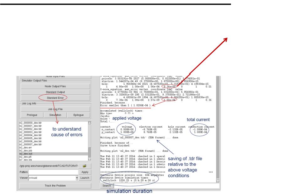
Simulation output file
• Select Standard Output to explore:
–Host name (ex. bue), process ID (ex. 1512)
–used models and material parameters
–monitoring of the boundary conditions (like bias sweeps)
–information about numerical convergence
Error column: indication of convergence.
It is a “normalized” error indication. Convergence is achieved if error is smaller than one.
The coordinate of maximum error for each equation is also specified thanks to the use of the keyword
CNormPrint in the Sdevice command file. This information is particularly useful in case of nonconvergence, since it gives indication of where the numerical mesh could need revision
G. Betti Beneventi 30