

Young - Computational chemistry
.pdf20 3 AB INITIO METHODS
The Gaussian functions are multiplied by an angular function in order to give the orbital the symmetry of a s, p, d, and so on. A constant angular term yields s symmetry. Angular terms of x, y, z give p symmetry. Angular terms of xy, xz, yz, x2ÿy2, 4z2ÿ2x2ÿ2y2 yield d symmetry. This pattern can be continued for the other orbitals.
These orbitals are then combined into a determinant. This is done to satisfy two requirements of quantum mechanics. One is that the electrons must be indistinguishable. By having a linear combination of orbitals in which each electron appears in each orbital, it is only possible to say that an electron was put in a particular orbital but not which electron it is. The second requirement is that the wave function for fermions (an electron is a fermion) must be antisymmetric with respect to interchanging two particles. Thus, if electron 1 and electron 2 are switched, the sign of the total wave function must change and only the sign can change. This is satis®ed by a determinant because switching two electrons is equivalent to interchanging two columns of the determinant, which changes its sign.
The functions put into the determinant do not need to be individual GTO functions, called Gaussian primitives. They can be a weighted sum of basis functions on the same atom or di¨erent atoms. Sums of functions on the same atom are often used to make the calculation run faster, as discussed in Chapter 10. Sums of basis functions on di¨erent atoms are used to give the orbital a particular symmetry. For example, a water molecule with C2v symmetry will have orbitals that transform as A1, A2, B1, B2, which are the irreducible representations of the C2v point group. The resulting orbitals that use functions from multiple atoms are called molecular orbitals. This is done to make the calculation run much faster. Any overlap integral over orbitals of di¨erent symmetry does not need to be computed because it is zero by symmetry.
The steps in a Hartree±Fock calculation start with an initial guess for the orbital coe½cients, usually using a semiempirical method. This function is used to calculate an energy and a new set of orbital coe½cients, which can then be used to obtain a new set, and so on. This procedure continues iteratively until the energies and orbital coe½cients remain constant from one iteration to the next. This is called having the calculation converge. There is no guarantee the calculation will converge. In cases where it does not, some technical expertise is required to ®x the problem, as discussed in Chapter 22. This iterative procedure is called a self-consistent ®eld procedure (SCF). Some researchers refer to these as SCF calculations to distinguish them from the earlier method created by Hartree, but HF is used more widely.
A variation on the HF procedure is the way that orbitals are constructed to re¯ect paired or unpaired electrons. If the molecule has a singlet spin, then the same orbital spatial function can be used for both the a and b spin electrons in each pair. This is called the restricted Hartree±Fock method (RHF).
There are two techniques for constructing HF wave functions of molecules with unpaired electrons. One technique is to use two completely separate sets of orbitals for the a and b electrons. This is called an unrestricted Hartree±Fock
3.2 CORRELATION 21
wave function (UHF). This means that paired electrons will not have the same spatial distribution. This introduces an error into the calculation, called spin contamination. Spin contamination might introduce an insigni®cant error or the error could be large enough to make the results unusable depending on the chemical system involved. Spin contamination is discussed in more detail in Chapter 27. UHF calculation are popular because they are easy to implement and run fairly e½ciently.
Another way of constructing wave functions for open-shell molecules is the restricted open shell Hartree±Fock method (ROHF). In this method, the paired electrons share the same spatial orbital; thus, there is no spin contamination. The ROHF technique is more di½cult to implement than UHF and may require slightly more CPU time to execute. ROHF is primarily used for cases where spin contamination is large using UHF.
For singlet spin molecules at the equilibrium geometry, RHF and UHF wave functions are almost always identical. RHF wave functions are used for singlets because the calculation takes less CPU time. In a few rare cases, a singlet molecule has biradical resonance structures and UHF will give a better description of the molecule (i.e., ozone).
The RHF scheme results in forcing electrons to remain paired. This means that the calculation will fail to re¯ect cases where the electrons should uncouple. For example, a series of RHF calculations for H2 with successively longer bond lengths will show that H2 dissociates into H‡ and Hÿ, rather than two H atoms. This limitation must be considered whenever processes involving pairing and unpairing of electrons are modeled. This is responsible for certain systematic errors in HF results, such as activation energies that are too high, bond lengths slightly too short, vibrational frequencies too high, and dipole moments and atomic charges that are too large. UHF wave functions usually dissociate correctly.
There are a number of other technical details associated with HF and other ab initio methods that are discussed in other chapters. Basis sets and basis set superposition error are discussed in more detail in Chapters 10 and 28. For openshell systems, additional issues exist: spin polarization, symmetry breaking, and spin contamination. These are discussed in Chapter 27. Size±consistency and size±extensivity are discussed in Chapter 26.
3.2CORRELATION
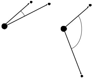
One of the limitations of HF calculations is that they do not include electron correlation. This means that HF takes into account the average a¨ect of electron repulsion, but not the explicit electron±electron interaction. Within HF theory the probability of ®nding an electron at some location around an atom is determined by the distance from the nucleus but not the distance to the other electrons as shown in Figure 3.1. This is not physically true, but it is the consequence of the central ®eld approximation, which de®nes the HF method.
22 3 AB INITIO METHODS
θ1 |
r1 |
r1 |
r2 |
|
θ2
r2
FIGURE 3.1 Two arrangements of electrons around the nucleus of an atom having the same probability within HF theory, but not in correlated calculations.
A number of types of calculations begin with a HF calculation and then correct for correlation. Some of these methods are Mùller±Plesset perturbation theory (MPn, where n is the order of correction), the generalized valence bond (GVB) method, multi-con®gurational self-consistent ®eld (MCSCF), con®guration interaction (CI), and coupled cluster theory (CC). As a group, these methods are referred to as correlated calculations.
Correlation is important for many di¨erent reasons. Including correlation generally improves the accuracy of computed energies and molecular geometries. For organic molecules, correlation is an extra correction for very-high- accuracy work, but is not generally needed to obtain quantitative results. One exception to this rule are compounds exhibiting Jahn±Teller distortions, which often require correlation to give quantitatively correct results. An extreme case is transition metal systems, which often require correlation in order to obtain results that are qualitatively correct.
3.3MéLLER±PLESSET PERTURBATION THEORY
Correlation can be added as a perturbation from the Hartree±Fock wave function. This is called Mùller±Plesset perturbation theory. In mapping the HF wave function onto a perturbation theory formulation, HF becomes a ®rst-order perturbation. Thus, a minimal amount of correlation is added by using the secondorder MP2 method. Third-order (MP3) and fourth-order (MP4) calculations are also common. The accuracy of an MP4 calculation is roughly equivalent to the accuracy of a CISD calculation. MP5 and higher calculations are seldom done due to the high computational cost (N 10 time complexity or worse).
3.4 CONFIGURATION INTERACTION |
23 |
Energy
exact
MP2 |
MP3 |
MP4 |
MP5 |
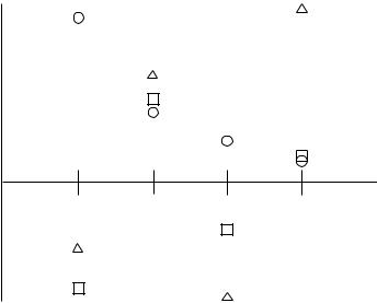
FIGURE 3.2 Possible results of increasing the order of Mùller±Plesset calculations. The circles show monotonic convergence. The squares show oscillating convergence. The triangles show a diverging series.
Mùller±Plesset calculations are not variational. In fact, it is not uncommon to ®nd MP2 calculations that give total energies below the exact total energy. Depending on the nature of the chemical system, there seem to be two patterns in using successively higher orders of perturbation theory. For some systems, the energies become successively lower and closer to the total energy in going from MP2 to MP3, to MP4, and so on, as shown in Figure 3.2. For other systems, MP2 will have an energy lower than the exact energy, MP3 will be higher, MP4 will be lower, and so on, with each having an error that is lower in magnitude but opposite in sign. If the assumption of a small perturbation is not valid, the MPn energies may diverge as shown in Figure 3.2. This might happen if the single determinant reference is a poor qualitative description of the system. One advantage of Mùller±Plesset is that it is size extensive.
There is also a local MP2 (LMP2) method. LMP2 calculations require less CPU time than MP2 calculations. LMP2 is also less susceptible to basis set superposition error. The price of these improvements is that about 98% of the MP2 energy correction is recovered by LMP2.
3.4CONFIGURATION INTERACTION
A con®guration interaction wave function is a multiple-determinant wave function. This is constructed by starting with the HF wave function and making new determinants by promoting electrons from the occupied to unoccupied or-
24 3 AB INITIO METHODS
bitals. Con®guration interaction calculations can be very accurate, but the cost in CPU time is very high (N 8 time complexity or worse).
Con®guration interaction calculations are classi®ed by the number of excitations used to make each determinant. If only one electron has been moved for each determinant, it is called a con®guration interaction single-excitation (CIS) calculation. CIS calculations give an approximation to the excited states of the molecule, but do not change the ground-state energy. Single-and doubleexcitation (CISD) calculations yield a ground-state energy that has been corrected for correlation. Triple-excitation (CISDT) and quadruple-excitation (CISDTQ) calculations are done only when very-high-accuracy results are desired.
The con®guration interaction calculation with all possible excitations is called a full CI. The full CI calculation using an in®nitely large basis set will give an exact quantum mechanical result. However, full CI calculations are very rarely done due to the immense amount of computer power required.
CI results can vary a little bit from one software program to another for open-shell molecules. This is because of the HF reference state being used. Some programs, such as Gaussian, use a UHF reference state. Other programs, such as MOLPRO and MOLCAS, use a ROHF reference state. The di¨erence in results is generally fairly small and becomes smaller with higher-order calculations. In the limit of a full CI, there is no di¨erence.
3.5MULTI-CONFIGURATIONAL SELF-CONSISTENT FIELD
MCSCF calculations also use multiple determinants. However, in an MCSCF calculation the orbitals are optimized for use with the multiple-determinant wave function. These calculations can often give the most accurate results for a given amount of CPU time. Compared to a CI calculation, an MCSCF gives more of the correlation energy with fewer con®gurations. However, CI calculations usually give more correlation energy in total because so many more con®gurations are included.
It is particularly desirable to use MCSCF or MRCI if the HF wave function yield a poor qualitative description of the system. This can be determined by examining the weight of the HF reference determinant in a single-reference CI calculation. If the HF determinant weight is less than about 0.9, then it is a poor description of the system, indicating the need for either a multiplereference calculation or triple and quadruple excitations in a single-reference calculation.
Unfortunately, these methods require more technical sophistication on the part of the user. This is because there is no completely automated way to choose which con®gurations are in the calculation (called the active space). The user must determine which molecular orbitals to use. In choosing which orbitals to include, the user should ensure that the bonding and corresponding antibonding orbitals are correlated. The orbitals that will yield the most correlation
3.7 COUPLED CLUSTER |
25 |
energy can be determined by running an unrestricted or correlated calculation, then using the ``virtual'' natural orbitals with the highest occupation numbers along with their corresponding ``occupied'' orbitals. If the orbitals are chosen poorly, as is almost always the case without manual intervention, the results will not only fail to improve, but also they may actually become less accurate with the addition of more orbitals.
An MCSCF calculation in which all combinations of the active space orbitals are included is called a complete active space self-consistent ®eld (CASSCF) calculation. This type of calculation is popular because it gives the maximum correlation in the valence region. The smallest MCSCF calculations are twocon®guration SCF (TCSCF) calculations. The generalized valence bond (GVB) method is a small MCSCF including a pair of orbitals for each molecular bond.
3.6MULTI-REFERENCE CONFIGURATION INTERACTION
It is possible to construct a CI wave function starting with an MCSCF calculation rather than starting with a HF wave function. This starting wave function is called the reference state. These calculations are called multi-reference con®guration interaction (MRCI) calculations. There are more CI determinants in this type of calculation than in a conventional CI. This type of calculation can be very costly in terms of computing resources, but can give an optimal amount of correlation for some problems.
The notation for denoting this type of calculation is sometimes more speci®c. For example, the acronym MCSCF‡1‡2 means that the calculation is a MRCI calculation with single and double CI excitations out of an MCSCF reference space. Likewise, CASSCF‡1‡2 and GVB‡1‡2 calculations are possible.
3.7COUPLED CLUSTER
Coupled cluster calculations are similar to con®guration interaction calculations in that the wave function is a linear combination of many determinants. However, the means for choosing the determinants in a coupled cluster calculation is more complex than the choice of determinants in a CI. Like CI, there are various orders of the CC expansion, called CCSD, CCSDT, and so on. A calculation denoted CCSD(T) is one in which the triple excitations are included perturbatively rather than exactly.
Coupled cluster calculations give variational energies as long as the excitations are included successively. Thus, CCSD is variational, but CCD is not. CCD still tends to be a bit more accurate than CID.
The accuracy of these two methods is very similar. The advantage of doing coupled cluster calculations is that it is a size extensive method (see chapter 26). Often, coupled-cluster results are a bit more accurate than the equivalent
26 3 AB INITIO METHODS
size con®guration interaction calculation results. When all possible con®gurations are included, a full coupled-cluster calculation is equivalent to a full CI calculation.
Quadratic con®guration interaction calculations (QCI) use an algorithm that is a combination of the CI and CC algorithms. Thus, a QCISD calculation is an approximation to a CCSD calculation. These calculations are popular since they often give an optimal amount of correlation for high-accuracy calculations on organic molecules while using less CPU time than coupled cluster calculations. Most popular is the singleand double-excitation calculation, QCISD. Sometimes, triple excitations are included as well, QCISD(T). The T in parentheses indicates that the triple excitations are included perturbatively.
There is a variation on the coupled cluster method known as the symmetry adapted cluster (SAC) method. This is also a size consistent method. For excited states, a CI out of this space, called a SAC-CI, is done. This improves the accuracy of electronic excited-state energies.
Another technique, called Brueckner doubles, uses orbitals optimized to make single excitation contributions zero and then includes double excitations. This is essentially equivalent to CCSD in terms of both accuracy and CPU time.
3.8QUANTUM MONTE CARLO METHODS
A method that avoids making the HF mistakes in the ®rst place is called quantum Monte Carlo (QMC). There are several types of QMC: variational, di¨usion, and Greens function Monte Carlo calculations. These methods work with an explicitly correlated wave function. This is a wave function that has a function of the electron±electron distance (a generalization of the original work by Hylleraas).
The wave function for a variational QMC calculation might take the functional form
Y |
…3:1† |
C ˆ DaDb f …rij† |
|
i< j |
|
where Da and Db are determinants of a and b spin electrons. The use of two determinants in this way does not introduce any additional error as long as there are not any spin terms in the Hamiltonian (i.e., spin coupling). The f …rij † term is the term that accounts for electron correlation. This correlation function could include three body terms, denoted f …ri; rj; rij †. The general shape of the correlation function is known, but there is not yet a consensus on the best mathematical function to use and new functions are still being proposed.
The di¨usion and Greens function Monte Carlo methods use numerical wave functions. In this case, care must be taken to ensure that the wave function has the nodal properties of an antisymmetric function. Often, nodal sur-
3.10 CONCLUSIONS 27
faces from HF wave functions are used. In the most sophisticated calculations, the nodal surfaces are ``relaxed,'' meaning that they are allowed to shift to optimize the wave function.
The integrals over the wave function are evaluated numerically using a Monte Carlo integration scheme. These calculations can be extremely time-consuming, but they are probably the most accurate methods known today. Because these calculations scale as N 3 and are extremely accurate, it is possible they could become important in the future if they can be made faster. At this current stage of development, most of the researchers using quantum Monte Carlo calculations are those writing their own computer codes and inventing the methods contained therein.
3.9NATURAL ORBITALS
Once an energy and wave function has been found, it is often necessary to compute other properties of the molecule. For the multiple-determinant methods (MCSCF, CI, CC, MRCI), this is done most e½ciently using natural orbitals. Natural orbitals are the eigenfunctions of the ®rst-order reduced density matrix. The details of density matrix theory are beyond the scope of this text. Su½ce it to say that once the natural orbitals have been found, the information in the wave function has been compressed from a many-determinant function down to a set of orbitals and occupation numbers. The occupation numbers are the number of electrons in each natural orbital. This is a real number, which is close to one or two electrons for those considered to be occupied orbitals. Many of the higher-energy orbitals have a small amount of electron occupation, which is roughly analogous to the excited-con®guration weights in the wave function, but not mathematically equivalent.
Properties can be computed by ®nding the expectation value of the property operator with the natural orbitals weighted by the occupation number of each orbital. This is a much faster way to compute properties than trying to use the expectation value of a multiple-determinant wave function. Natural orbitals are not equivalent to HF or Kohn±Sham orbitals, although the same symmetry properties are present.
3.10CONCLUSIONS
In general, ab initio calculations give very good qualitative results and can yield increasingly accurate quantitative results as the molecules in question become smaller. The advantage of ab initio methods is that they eventually converge to the exact solution once all the approximations are made su½ciently small in magnitude. In general, the relative accuracy of results is
HF f MP2 < CISD G MP4 G CCSD < CCSD…T† < CCSDT < Full CI
28 3 AB INITIO METHODS
However, this convergence is not monotonic. Sometimes, the smallest calculation gives a very accurate result for a given property. There are four sources of error in ab initio calculations:
1.The Born±Oppenheimer approximation
2.The use of an incomplete basis set
3.Incomplete correlation
4.The omission of relativistic e¨ects
The disadvantage of ab initio methods is that they are expensive. These methods often take enormous amounts of computer CPU time, memory, and disk space. The HF method scales as N 4, where N is the number of basis functions. This means that a calculation twice as big takes 16 times as long …24† to complete. Correlated calculations often scale much worse than this. In practice, extremely accurate solutions are only obtainable when the molecule contains a dozen electrons or less. However, results with an accuracy rivaling that of many experimental techniques can be obtained for moderate-size organic molecules. The minimally correlated methods, such as MP2 and GVB, are often used when correlation is important to the description of large molecules.
BIBLIOGRAPHY
Some textbooks discussing ab initio methods are
F.Jensen, Introduction to Computational Chemistry John Wiley & Sons, New York (1999).
T.VeszpreÂmi, M. FeheÂr, Quantum Chemistry; Fundamentals to Applications Kluwer, Dordrecht (1999).
D. B. Cook, Handbook of Computational Quantum Chemistry Oxford, Oxford (1998).
P. W. Atkins, R. S. Friedman, Molecular Quantum Mechanics Oxford, Oxford (1997).
J. Simons, J. Nichols, Quantum Mechanics in Chemistry Oxford, Oxford (1997).
A. R. Leach, Molecular Modelling Principles and Applications Longman, Essex (1996).
P.Fulde, Electron Correlations in Molecules and Solids Third Enlarged Edition Springer, Berlin (1995).
B.L. Hammond, W. A. Lester, Jr., P. J. Reynolds, Monte Carlo Methods in Ab Initio Quantum Chemistry World Scienti®c, Singapore (1994).
I. N. Levine, Quantum Chemistry Prentice Hall, Englewood Cli¨s (1991).
T.Clark, A Handbook of Computational Chemistry John Wiley & Sons, New York (1985).
S. Wilson, Electron Correlation in Molecules Clarendon, Oxford (1984).
D. A. McQuarrie, Quantum Chemistry University Science Books, Mill Valley (1983).
BIBLIOGRAPHY 29
A. C. Hurley, Electron Correlation in Small Molecules Academic Press, London (1976).
Articles reviewing ab initio methods in general, or topics common to all methods
E. R. Davidson, Encycl. Comput. Chem. 3, 1811 (1998).
S.Profeta, Jr., Kirk-Othmer Encyclopedia of Chemical Technology Supplement 315, J. I. Kroschwitz Ed. John Wiley & Sons, New York (1998).
S. Shaik, Encycl. Comput. Chem. 5, 3143 (1998).
S. Sabo-Etienne, B. Chaudret, Chem. Rev. 98, 2077 (1998).
J. Gerratt, D. L. Cooper, P. B. Karadakov, M. Raimond, Chem. Soc. Rev. 26, 87 (1997).
Adv. Chem. Phys. vol 93 (1996).
J. Cioslowski, Rev. Comput. Chem. 4, 1 (1993).
R. A. Friesner, Ann. Rev. Phys. Chem. 42, 341 (1991).
D. L. Cooper, J. Gerratt, M. Raimondi, Chem. Rev. 91, 929 (1991).
Adv. Chem. Phys. vol. 69 (1987).
G. Marc, W. G. McMillan, Adv. Chem. Phys. 58, 209 (1985).
G. A. Gallup, R. L. Vance, J. R. Collins, J. M. Norbeck, Adv. Quantum Chem. 16, 229 (1982).
H. F. Schaefer, III, Ann. Rev. Phys. Chem. 27, 261 (1976). E. R. Davidson, Adv. Quantum Chem. 6, 235 (1972).
H. A. Bent, Chem. Rev. 61, 275 (1961).
Sources comparing the accuracy of results are
F. Jensen, Introduction to Computational Chemistry John Wiley & Sons, New York (1999).
H. Partridge, Encycl. Comput. Chem. 1, 581 (1998).
J.B. Foresman, á. Frisch, Exploring Chemistry with Electronic Structure Methods
Gaussian, Pittsburgh (1996).
K.Raghavachari, J. B. Anderson, J. Phys. Chem. 100, 12960 (1996).
R.J. Bartlett, Modern Electronic Structure Theory Part 2 D. R. Yarkony, Ed., 1047, World Scienti®c, Singapore (1995).
T.J. Lee, G. E. Scuseria, Quantum Mechanical Electronic Structure Calculations with Chemical Accuracy S. R. Langho¨, Ed., 47, Kluwer, Dordrecht (1995).
W. J. Hehre, Practical Strategies for Electronic Structure Calculations Wavefunction, Irvine (1995).
H. F. Schaefer, III, J. R. Thomas, Y. Yamaguchi, B. J. DeLeeuw, G. Vacek, Modern Electronic Structure Theory Part 1 D. R. Yarkony, Ed., 3, World Scienti®c, Singapore (1995).
C. W. Bauschlicker, Jr., S. R. Langho¨, P. R. Taylor, Adv. Chem. Phys. 77, 103 (1990).
W. J. Hehre, L. Radom, P. v.R. Schleyer, J. A. Pople, Ab Initio Molecular Orbital Theory John Wiley & Sons, New York (1986).
V. KvasnicÏka, V. Laurinc, S. BiskupicÏ, M. Haring, Adv. Chem. Phys. 52, 181 (1983).