Young - Computational chemistry

10 2 FUNDAMENTAL PRINCIPLES

and the general inability to provide detailed insight into chemical processes. Very often, any thermodynamic treatment is left for trivial pen-and-paper work since many aspects of chemistry are so accurately described with very simple mathematical expressions.

Computational results can be related to thermodynamics. The result of computations might be internal energies, free energies, and so on, depending on the computation done. Likewise, it is possible to compute various contributions to the entropy. One frustration is that computational software does not always make it obvious which energy is being listed due to the di¨erences in terminology between computational chemistry and thermodynamics. Some of these di¨erences will be noted at the appropriate point in this book.

2.5QUANTUM MECHANICS

Quantum mechanics (QM) is the correct mathematical description of the behavior of electrons and thus of chemistry. In theory, QM can predict any property of an individual atom or molecule exactly. In practice, the QM equations have only been solved exactly for one electron systems. A myriad collection of methods has been developed for approximating the solution for multiple electron systems. These approximations can be very useful, but this requires an amount of sophistication on the part of the researcher to know when each approximation is valid and how accurate the results are likely to be. A signi®- cant portion of this book addresses these questions.

Two equivalent formulations of QM were devised by SchroÈdinger and Heisenberg. Here, we will present only the SchroÈdinger form since it is the basis for nearly all computational chemistry methods. The SchroÈdinger equation is

^	…2:4†
HC ˆ EC

where ^ is the Hamiltonian operator, C a wave function, and the energy. In

H E

the language of mathematics, an equation of this form is called an eigen equation. C is then called the eigenfunction and E an eigenvalue. The operator and eigenfunction can be a matrix and vector, respectively, but this is not always the case.

The wave function C is a function of the electron and nuclear positions. As the name implies, this is the description of an electron as a wave. This is a probabilistic description of electron behavior. As such, it can describe the probability of electrons being in certain locations, but it cannot predict exactly where electrons are located. The wave function is also called a probability amplitude because it is the square of the wave function that yields probabilities. This is the only rigorously correct meaning of a wave function. In order to obtain a physically relevant solution of the SchroÈdinger equation, the wave function must be continuous, single-valued, normalizable, and antisymmetric with respect to the interchange of electrons.

2.5 QUANTUM MECHANICS 11

The Hamiltonian operator ^ is, in general,

H

particles

`2

particles

qiqj

^

X

i

X X

H

ˆ ÿ

i

2mi

‡

rij

…2:5†

i< j

`i2

q2

q2

q2

ˆ

‡

‡

…2:6†

qx2

qy2

qz2

i

i

i

where `i2 is the Laplacian operator acting on particle i. Particles are both electrons and nuclei. The symbols mi and qi are the mass and charge of particle i, and rij is the distance between particles. The ®rst term gives the kinetic energy of the particle within a wave formulation. The second term is the energy due to Coulombic attraction or repulsion of particles. This formulation is the timeindependent, nonrelativistic SchroÈdinger equation. Additional terms can appear in the Hamiltonian when relativity or interactions with electromagnetic radiation or ®elds are taken into account.

In currently available software, the Hamiltonian above is nearly never used. The problem can be simpli®ed by separating the nuclear and electron motions. This is called the Born±Oppenheimer approximation. The Hamiltonian for a molecule with stationary nuclei is

	X			X	X			X	X
^	electrons `i2			nuclei electrons Zi				electrons		1
H ˆ ÿ	i	2	ÿ	i	j	rij	‡	i< j		rij	…2:7†

Here, the ®rst term is the kinetic energy of the electrons only. The second term is the attraction of electrons to nuclei. The third term is the repulsion between electrons. The repulsion between nuclei is added onto the energy at the end of the calculation. The motion of nuclei can be described by considering this entire formulation to be a potential energy surface on which nuclei move.

Once a wave function has been determined, any property of the individual molecule can be determined. This is done by taking the expectation value of the operator for that property, denoted with angled brackets h i. For example, the energy is the expectation value of the Hamiltonian operator given by

…

h	E	i ˆ	C H^C	…	2:8	†

For an exact solution, this is the same as the energy predicted by the SchroÈdinger equation. For an approximate wave function, this gives an approximation of the energy, which is the basis for many of the techniques described in subsequent chapters. This is called variational energy because it is always greater than or equal to the exact energy. By substituting di¨erent operators, it is possible to obtain di¨erent observable properties, such as the dipole moment or electron density. Properties other than the energy are not variational, because

12 2 FUNDAMENTAL PRINCIPLES

only the Hamiltonian is used to obtain the wave function in the widely used computational chemistry methods.

Another way of obtaining molecular properties is to use the Hellmann± Feynman theorem. This theorem states that the derivative of energy with respect to some property P is given by

dP	ˆ	*qP+	…2:9†
dE		^
		qH

This relationship is often used for computing electrostatic properties. Not all approximation methods obey the Hellmann±Feynman theorem. Only variational methods obey the Hellmann±Feynman theorem. Some of the variational methods that will be discussed in this book are denoted HF, MCSCF, CI, and CC.

2.6STATISTICAL MECHANICS

Statistical mechanics is the mathematical means to calculate the thermodynamic properties of bulk materials from a molecular description of the materials. Much of statistical mechanics is still at the paper-and-pencil stage of theory. Since quantum mechanicians cannot exactly solve the SchroÈdinger equation yet, statistical mechanicians do not really have even a starting point for a truly rigorous treatment. In spite of this limitation, some very useful results for bulk materials can be obtained.

Statistical mechanics computations are often tacked onto the end of ab initio vibrational frequency calculations for gas-phase properties at low pressure. For condensed-phase properties, often molecular dynamics or Monte Carlo calculations are necessary in order to obtain statistical data. The following are the principles that make this possible.

Consider a quantity of some liquid, say, a drop of water, that is composed of N individual molecules. To describe the geometry of this system if we assume the molecules are rigid, each molecule must be described by six numbers: three to give its position and three to describe its rotational orientation. This 6Ndimensional space is called phase space. Dynamical calculations must additionally maintain a list of velocities.

An individual point in phase space, denoted by G, corresponds to a particular geometry of all the molecules in the system. There are many points in this phase space that will never occur in any real system, such as con®gurations with two atoms in the same place. In order to describe a real system, it is necessary to determine what con®gurations could occur and the probability of their occurrence.

The probability of a con®guration occurring is a function of the energy of that con®guration. This energy is the sum of the potential energy from inter-

2.6 STATISTICAL MECHANICS

13

molecular attractive or repulsive forces and the kinetic energy due to molecular motion. For an ideal gas, only the kinetic energy needs to be considered. For a molecular gas, the kinetic energy is composed of translational, rotational, and vibrational motion. For a monatomic ideal gas, the energy is due to the translational motion only. For simplicity of discussion, we will refer to the energy of the system or molecule without di¨erentiating the type of energy.

There is a di¨erence between the energy of the system, composed of all molecules, and the energy of the individual molecules. There is an amount of energy in the entire system that is measurable as the temperature of the system. However, not all molecules will have the same energy. Individual molecules will have more or less energy, depending on their motion and interaction with other molecules. There is some probability of ®nding molecules with any given energy. This probability depends on the temperature T of the system. The function that gives the ratio of the number of molecules, Ni, with various energies, Ei, to the number of molecules in state j is the Boltzmann distribution, which is expressed as

Ni	ˆ eÿ…Ei ÿEj †=kBT	…2:10†
Nj

where kB is the Boltzmann constant, 1:38066 10ÿ23 J/K.

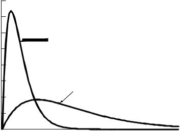
Equation (2.10) is valid if there are an equal number of ways to put the system in both energy states. Very often, there are more states available with higher energies due to there being an increasing number of degenerate states. When this occurs, the percentage of molecules in each state is determined by multiplying the equation above by the number of states available. Thus, there is often a higher probability of ®nding high-energy molecules at higher temperatures as shown in Figure 2.1. Note that the ground state may be a very poor approximation to the average.

When some property of a system is measured experimentally, the result is an average for all of the molecules with their respective energies. This observed quantity is a statistical average, called a weighted average. It corresponds to the result obtained by determining that property for every possible energy state of the system, A…G†, and multiplying by the probability of ®nding the system in that energy state, w…G†. This weighted average must be normalized by a parti-

tion function Q, where	P w…Q†A…G†
hAi ˆ		…2:11†
	G
Q ˆ X w…G†		…2:12†

This technique for ®nding a weighted average is used for ideal gas properties and quantum mechanical systems with quantized energy levels. It is not a convenient way to design computer simulations for real gas or condensed-phase

14 2 FUNDAMENTAL PRINCIPLES

	0.8
	0.7
	0.6
	low temperature
of molecules	0.5
	0.4
Fraction	0.3
	high temperature
	0.2
	0.1
	0.0
	Energy

FIGURE 2.1 Fraction of molecules that will be found at various energies above the ground-state energy for two di¨erent temperatures.

systems, because determining every possible energy state is by no means a trivial task. However, a result can be obtained from a reasonable sampling of states. This results in values having a statistical uncertainty s that is related to the number of states sampled M by

	••••••	…	2:13	†
	M
sa p1

There could also be systematic errors that are not indicated by this relationship. Another way of formulating this problem is to use derivatives of the partition function without a weight function. This is done with the following rela-

tionships:

		q ln Q
U ˆ kBT 2					V					…2:14†
		qT
A ˆ ÿkBT ln Q										…2:15†
q ln Q
P ˆ kBT				T						…2:16†
		qV
								q2 ln Q	V
CV ˆ 2kBT		q ln	Q				‡ kBT 2		!	…2:17†
		qT				V		qT 2

							2.6 STATISTICAL MECHANICS			15
		q ln Q						q ln Q
H ˆ kBT 2					V		‡ kBTV		T	…2:18†
			qT					qV
q ln Q
S ˆ kBT				V ‡ kB ln Q						…2:19†
		qT
		q ln Q
G ˆ kBTV						T	ÿ kBT ln Q			…2:20†
			qV

Other thermodynamic functions can be computed from these quantities. This is still not an ideal way to compute properties due to the necessity of accounting for all energy states of the system in order to obtain Q.

It is hardest to obtain precise values for the enthalpic values A, S, and G because they depend more heavily on high-energy states, which the system achieves infrequently. These functions depend on the actual value of Q, not just its derivatives.

There are several other, equivalent ways to obtain a statistical average. One of these is to use a time average. In this formulation, a calculation is designed to simulate the motion of molecules. At every step in the simulation, the property is computed for one molecule and averaged over all the time steps equally. This is equivalent to the weighted average because the molecule will be in more probable energy states a larger percentage of the time. The accuracy of this result depends on the number of time steps and the ability of the simulation to correctly describe how the real system will behave.

Another averaging technique is an ensemble average. Simulations often include thousands of molecules. A value can be averaged by including the result for every molecule in the simulation. This corresponds to the concept of an ensemble of molecules and is thus called an ensemble average. It is often most e½cient to combine time averages and ensemble averages, thus averaging all molecules over many time steps.

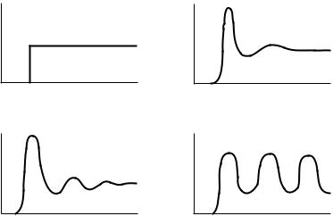
Another type of property to examine is the geometric orientation of molecules. A set of Cartesian coordinates will describe a point in phase space, but it does not convey the statistical tendency of molecules to orient in a certain way. This statistical description of geometry is given by a radial distribution function, also called a pair distribution function. This is the function that gives the probability of ®nding atoms various distances apart. The radial distribution function gives an indication of phase behavior as shown in Figure 2.2. More detail can be obtained by using atom-speci®c radial distribution functions, such as the probability of ®nding a hydrogen atom various distances from an oxygen atom.

The connections between simulation and thermodynamics can be carried further. Simulations can be set up to be constant volume, pressure, temperature, and so on. Some of the most sophisticated simulations are those involving multiple phases or phase changes. These techniques are discussed further in Chapter 7.

16 2 FUNDAMENTAL PRINCIPLES
(a)	(b)
g(r)	g(r)
r	r
(c)	(d)
g(r)	g(r)
r	r

FIGURE 2.2 Radial distribution functions for (a) a hard sphere ¯uid, (b) a real gas, (c) a liquid, (d ) a crystal.

BIBLIOGRAPHY

Sources covering fundamental principles are

T. P. Straatsma, J. A. McCammon, Ann. Rev. Phys. Chem. 43, 407 (1992).

D. Halliday, R. Resnick, Fundamentals of Physics John Wiley & Sons, New York (1988).

R.P. Feynman, R. B. Leighton, M. Sands, The Feynman Lectures on Physics AddisonWesley, Reading (1963).

A review of the implications of electrostatics is

G.NaÂray-SzaboÂ, G. G. Ferency, Chem. Rev. 95, 829 (1995).

Some texts covering thermodynamics are

I.N. Levine, Physical Chemistry McGraw-Hill, New York (1995).

J.W. Whalen, Molecular Thermodynamics: A Statistical Approach John Wiley & Sons, NY (1991).

P.W. Atkins, Physical Chemistry W. H. Freeman, New York (1990). T. L. Hill, Thermodynamics of Small Systems Dover, New York (1964).

Some quantum mechanics texts are

J. E. House, Fundamentals of Quantum Mechanics Academic Press, San Diego (1998). P. W. Atkins, R. S. Friedman, Molecular Quantum Mechanics Oxford, Oxford (1997).

BIBLIOGRAPHY 17

J.Simons, J. Nichols, Quantum Mechanics in Chemistry Oxford, Oxford (1997). R. H. Landau, Quantum Mechanics II John Wiley & Sons, New York (1996). A. Szabo, N. S. Ostlund, Modern Quantum Chemistry Dover, New York (1996). W. Greiner, Quantum Mechanics An Introduction Springer, Berlin (1994).

J. P. Lowe, Quantum Chemistry Academic Press, San Diego (1993). P. W. Atkins, Quanta Oxford, Oxford (1991).

I. N. Levine, Quantum Chemistry Prentice Hall, Englewood Cli¨s (1991).

R. E. Christo¨ersen, Basic Principles and Techniques of Molecular Quantum Mechanics

Springer-Verlag, New York (1989).

D. A. McQuarrie Quantum Chemistry University Science Books, Mill Valley, CA (1983).

D. Bohm, Quantum Theory Dover, New York (1979).

C.Cohen-Tannoudji, B. Diu, F. LaloeÈ, Quantum Mechanics Wiley-Interscience, New York (1977).

R. McWeeny, B. T. Sutcli¨e, Methods of Molecular Quantum Mechanics Academic Press, London (1976).

E. Merzbacher, Quantum Mechanics John Wiley & Sons, New York (1970).

L.Pauling, E. B. Wilson, Jr., Introduction to Quantum Mechanics With Applications to Chemistry Dover, New York (1963).

P.A. M. Dirac, The Principles of Quantum Mechanics Oxford, Oxford (1958).

Some overviews of statistical mechanics are

A.Maczek, Statistical Thermodynamics Oxford, Oxford (1998).

J. Goodisman, Statistical Mechanics for Chemists John Wiley & Sons, New York (1997). R. E. Wilde, S. Singh, Statistical Mechanics: Fundamentals and Modern Applications

John Wiley & Sons, New York (1997).

D. Frenkel, B. Smit, Understanding Molecular Simulations Academic Press, San Diego (1996).

C.Garrod, Statistical Mechanics and Thermodynamics Oxford, Oxford (1995).

G.Jolicard, Ann. Rev. Phys. Chem. 46, 83 (1995).

M.P. Allen, D. J. Tildesley, Computer Simulation of Liquids Oxford, Oxford (1987).

D.G. Chandler, Introduction to Modern Statistical Mechanics Oxford, Oxford (1987).

T.L. Hill, An Introduction to Statistical Thermodynamics Dover, New York (1986).

G.Sperber, Adv. Quantum Chem. 11, 411 (1978).

D.A. McQuarrie, Statistical Mechanics Harper Collins, New York (1976).

W.Forst, Chemn. Rev. 71, 339 (1971).

Adv. Chem. Phys. vol. 11 (1967).

E.SchroÈdinger, Statistical Thermodynamics Dover, New York (1952).

Implications of the Born-Oppenheimer approximation are reviewed in

P.M. Kozlowski, L. Adamowicz, Chem. Rev. 93, 2007 (1993).

18 2 FUNDAMENTAL PRINCIPLES

Computation of free energies is reviewed in

D. A. Pearlman, B. G. Rao, Encycl. Comput. Chem. 2, 1036 (1998). T. P. Straatsma, Encycl. Comput. Chem. 2, 1083 (1998).

T. P. Straatsma, Rev. Comput. Chem. 9, 81 (1996).

Path integral formulations of statistical mechanics are reviewed in

B. J. Berne, D. Thirumalai, Ann. Rev. Phys. Chem. 37, 401 (1986).

Simulation and prediction of phase changes is reviewed in

G. H. Fredrickson, Ann. Rev. Phys. Chem. 39, 149 (1988). A. D. J. Haymet, Ann. Rev. Phys. Chem. 38, 89 (1987). T. Kihara, Adv. Chem. Phys. 1, 267 (1958).

Computational Chemistry: A Practical Guide for Applying Techniques to Real-World Problems. David C. Young Copyright ( 2001 John Wiley & Sons, Inc.

ISBNs: 0-471-33368-9 (Hardback); 0-471-22065-5 (Electronic)

3 Ab initio Methods

The term ab initio is Latin for ``from the beginning.'' This name is given to computations that are derived directly from theoretical principles with no inclusion of experimental data. This is an approximate quantum mechanical calculation. The approximations made are usually mathematical approximations, such as using a simpler functional form for a function or ®nding an approximate solution to a di¨erential equation.

3.1HARTREE±FOCK APPROXIMATION

The most common type of ab initio calculation is called a Hartree±Fock calculation (abbreviated HF), in which the primary approximation is the central ®eld approximation. This means that the Coulombic electron±electron repulsion is taken into account by integrating the repulsion term. This gives the average e¨ect of the repulsion, but not the explicit repulsion interaction. This is a variational calculation, meaning that the approximate energies calculated are all equal to or greater than the exact energy. The energies are calculated in units called Hartrees (1 Hartree ˆ 27.2116 eV). Because of the central ®eld approximation, the energies from HF calculations are always greater than the exact energy and tend to a limiting value called the Hartree±Fock limit as the basis set is improved.

One of the advantages of this method is that it breaks the many-electron SchroÈdinger equation into many simpler one-electron equations. Each oneelectron equation is solved to yield a single-electron wave function, called an orbital, and an energy, called an orbital energy. The orbital describes the behavior of an electron in the net ®eld of all the other electrons.

The second approximation in HF calculations is due to the fact that the wave function must be described by some mathematical function, which is known exactly for only a few one-electron systems. The functions used most often are linear combinations of Gaussian-type orbitals exp…ÿar2†, abbreviated GTO. The wave function is formed from linear combinations of atomic orbitals or, stated more correctly, from linear combinations of basis functions. Because of this approximation, most HF calculations give a computed energy greater than the Hartree±Fock limit. The exact set of basis functions used is often speci®ed by an abbreviation, such as STOÿ3G or 6ÿ311‡‡g**. Basis sets are discussed further in Chapters 10 and 28.

19