Standard deviation

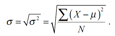
Negative and positive deviations should contribute equally to the characteristic variation. We use the fact that the squares of the two equal in magnitude numbers are equal, and calculate the mean squared deviation from the mean. This figure is called the variance and is denoted by σ2. The greater spread of values, the greater the variance. The dispersion was calculated by the formula:

As can be seen from the formula, the variance is measured in units of square units corresponding value. It's pretty uncomfortable. Therefore more likely to use the square root of the variance is the standard deviation σ

 

Normal distribution

Again referring to Fig. 1 and 2, we find that both planets increase of about 68% of the inhabitants do not differ from the average by more than one standard deviation, and about 95% - two standard deviations. Similar distributions are very common. We can say that this is what always happens when a certain value deviates from the average of the set under the influence of the weak, independent factors. Distribution of this kind is called normal (or Gaussian) and is described by the formula:

Note that the normal distribution is completely determined by the mean μ and standard deviation σ.

Medians and percentiles

Fig. 3. If the distribution is asymmetric to rely on the mean and standard deviation can not be. A. Distribution yupiterian on growth. B. The normal distribution with the same mean and standard deviation, in spite of the identity of the parameters, it did not look like a real distribution yupiterian.

Fig. 4. To describe the asymmetric distribution, use the median and percentiles. Median - the value that divides the distribution in half. A. The median growth yupiterian - 36 cm. B. 25 th and 75 th percentile cut off a quarter of the lowest and highest quarter yupiterian 25th percentile to the median is closer than 75 minutes - it speaks of asymmetric distribution.

Trusting the mean and standard deviation, we get a distorted picture of the population, are not normally distributed. To describe such data is better suited not mean and the median. The median - the value that divides the distribution in half half half the median values more -Less (more precisely not more).

  

Of course, the median and percentiles, unlike the mean and standard deviation, do not give a complete description of the distribution. However, between 25 th and 75 th percentiles is half the value - so we can tell what the average growth yupiterianin. On the situation with respect to the median of the 25th and 75th percentiles can be seen how an asymmetric distribution. Finally, now we know about who Jupiter is considered high (above the 75th percentile), and who did not come out growth (below the 25th percentile). Calculating percentile - a good way to understand how the distribution is close to normal. Recall that for a normal distribution of 95% of values enclosed within two standard deviations from the mean, and 68% - within one standard deviation, median coincides with the average.

 

If a match between the percentiles and the deviation from the average is not too different from the above, the distribution is close to normal and it can be described using the mean and standard deviation.

So far we have been able to obtain data on all sites combined, so that we can accurately calculate the values of the mean, variance and standard deviation. In fact, examine all the objects together is rarely possible: generally satisfied with the study sample, suggesting that this sample reflects the properties of the set. Sample that reflects the properties of the set is called a representative. In dealing with the sample, we certainly do not know the exact values of the mean and standard deviation, but we can evaluate them. Estimation of the mean calculated from the sample is called the sample average. Denote the sample mean and is calculated as follows:

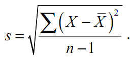
where n - sample size.

 

Fig. 5. This distribution is obtained by selecting 25 to 10 times the Martians from the set, and calculate the average for each sample. If you build rasppedelenie average for all possible samples, it would be normal. The mean of this distribution will be equal to the average of the population from which the sample is extracted. The standard deviation of this distribution is called the standard error of the mean - sX - is an estimate of the variability of the average values for the sample is a measure of the accuracy with which the sample mean X is an estimate of the average for the set of μ. Therefore SX is called a standard error of the mean.

If the variable is a sum of a large number of independent variables, it tends to a normal distribution, whatever the distribution of the variables forming the sum. Since the sample mean is determined precisely by this amount, it tends to the normal distribution, the greater the volume of the sample, the more accurate approximation. (If the sample belong together with a normal distribution, the distribution of sample means will be normal regardless of the volume of samples).

Average sample means will coincide with the average for the population.

The larger the sample, the more accurate estimate of the mean and the lower its standard error. The greater the variability of the initial population, the greater the variability of sample means, so the standard error of the mean increases with the standard deviation of the population.

The true standard error of the mean for a sample of size n, drawn from the totality of having a standard deviation σ, is equal to

 

Standard error - this is the best estimate of σX one sample:

where s - sample standard deviation.

The true average of the aggregate approximately 95% of cases is within 2 standard error of the sample mean.

As already mentioned, the distribution of sample means should always be approximately normal distribution regardless of the distribution of the population from which the sample extracted. This is the essence of the statement, called the central limit theorem. This theorem states the following:

-Vyborochnye Average have approximately normal distribution regardless of the initial distribution of the population from which the sample was drawn.

The average value of all possible sample means is an average of the original population.