Measurement and Control Basics 3rd Edition (complete book)

Chapter 2 – Process Control Loops

55

Integral action or reset action is the integration of the input error signal e over a very small time period dt. In effect, this means that for integral action, the value of the manipulated variable V is changed at a rate that is proportional to the amount of error e that exists for a given duration. In other words, integral control responds to the duration of the error as well as to its magnitude and direction. When the controlled variable is at the set point, the final control element remains stationary. In effect, this means that at steady state, when integral action is present there can be no offset; therefore, the steady-state error is zero.

This combination of proportional and integral action is called PI control. The control equation for PI control action is as follows:

		V = Kce +	Kc	t	edt	(2-41)
			t	∫
			i	0
where
Kc	=	the proportional gain
ti	=	the integral time
e	=	the error signal
V	=	controller output

The advantage of including the integral mode with the proportional mode is that the integral action eliminates offset. Typically, there is some decreased stability due to the presence of the integral mode. In other words, the addition of the integral action makes the total loop slightly less stable. One significant exception to this is in liquid flow control. Liquid flow control loops are extremely fast and tend to be very noisy. As a result, plants often add integral control to the feedback controller in liquid flow control loops to provide a dampening or filtering action for the loop. Of course, the advantage of eliminating any offset is still present, but this is not the principal motivating factor in such cases.

Tuning a PI controller is more difficult than tuning a simpler proportional controller. Two separate tuning adjustments must be made, and each depends on the other. The difficulty of tuning a controller increases dramatically with the number of adjustments that must be made.

It is conceivable to have a control action that is based solely on the rate of change or derivative of the error signal e. Although this is possible, it is not practical because, while the error might be large, if it were unchanging the controller output would be zero. Thus, rate control or derivative control is usually found in combination with proportional control. The equation for a proportional-derivative (PD) controller is as follows:

56 Measurement and Control Basics

	V = Kc e + Kctd	de	(2-42)
		dt

where td is the derivative time.

By adding derivative action to the controller, lead time is added in the controller to compensate for lag around the loop. Almost any process has a time delay or lag around the loop; therefore, the theoretical advantages of lead in the controller are appealing. However, it is a difficult control action to implement and adjust, and its usage is limited to cases of extensive lag in the process. This often occurs with large temperature-control systems. Taking the derivative of the error signal has the side effect of producing upsets whenever the set point is changed, so most controllers take the derivative of the process signal.

Adding derivative control to the controller makes the loop more stable if it is correctly tuned. Since the loop is more stable, the proportional gain may be higher, and it can thus decrease offset better than proportional action alone. It does not, of course, eliminate offset.

The equation for a three-mode controller, or PID (proportional-integral- derivative) controller, is as follows:

V = Kce +	K		t	+ Kctd	de
		c	∫ edt			(2-43)
	t	i			dt
			0

The three-mode control gives rapid response and exhibits no offset, but it is very difficult to tune because of the three terms that must be adjusted. As a result, it is used only in a very small number of applications, and operators often must adjust it extensively and continuously to keep it properly tuned. The PID mode, however, offers excellent control when proper tuning is used.

Five common types of control loops are encountered in process control: flow, level, temperature, analytical, and pressure. Table 2-2 provides basics guidelines for the controller modes that are generally used for each type of process control loop.

		Chapter 2 – Process Control Loops		57
Table 2-2. Guidelines for Selecting Controller Modes
Control Loop		Controller Mode
	Proportional	Integral	Derivative
Flow	Always	Usually	Never
Level	Always	Usually	Rarely
Temperature	Always	Usually	Usually
Analytical	Always	Usually	Sometimes
Pressure	Always	Usually	Sometimes

Performance Criteria

The final factor plants must consider before tuning a loop is the performance criteria that are to be used. There are four widely used criteria; each is based on a different method for minimizing the integral error of the deviation of measured control signal from the set point. The first three are the minimum integral of square error (ISE), the minimum integral of absolute error (IAE), and the minimum integral of absolute error multiplied by time (ITAE). In equation form, these three criteria are, respectively,

∞
ISE = ∫ e2 dt									(2-44)
0
∞
IAE = ∫		e				dt			(2-45)
0
∞
ITAE = ∫ t				e				dt	(2-46)
0

These three integral criteria methods are best suited for computer-based control applications. They are recommended only for such applications, where they can give excellent tuning and control results.

The fourth and most commonly used performance criterion was presented by J. G. Ziegler and N. B. Nichols at the annual meeting of the American Society of Mechanical Engineers in New York City in December 1941. It is known as the “Ziegler and Nichols one-quarter wave decay” criterion and is the basis of their tuning methods. A decay ratio of one-quarter means that the ratio of the overshoot of the first peak in the process response curve to the overshoot of the second peak is 4:1 (this is illustrated in Figure 2-20). Using a decay ratio of one-quarter represents a compromise between a rapid initial response and a fast return to the set point.

58 Measurement and Control Basics

Output
	Quarter wave = a/b = 1/4
	b
1.0	a
	P
0
0	Time

Figure 2-20. Process response curve for one-quarter decay ratio

Ziegler-Nichols Tuning Methods

Ziegler and Nichols called their tuning procedures the ultimate method because they required users to determine the ultimate gain and ultimate period for the closed control loop. The ultimate gain is the maximum allowable value of gain for a controller that has only a proportional mode in operation for which the closed-loop system shows a stable sine wave response to a disturbance.

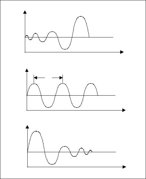
Suppose we have a closed-loop feedback control system that has the controller in the automatic mode, as shown in Figure 2-21c. If we increase the proportional gain the loop will tend to oscillate. If the gain is increased more, continuous cycling or oscillation in the controller output variable occur, as shown in Figure 2-21b. This is the maximum gain at which the system can be operated before it becomes unstable. This gain is called the ultimate gain or sensitivity (Su). The period of these sustained oscillations is called the ultimate period (Pu). If the gain is increased past this point, the system will become unstable, as shown in Figure 2-21a.

To determine the ultimate gain and the ultimate period, we perform the following steps:

1.Remove the reset and derivative action from the controller by setting the derivative time to zero, the reset time to infinity or the highest value possible, and the proportional gain to one.

2.Place the controller in automatic and make sure the loop is closed.

Chapter 2 – Process Control Loops

59

Output

(a) Unstable response	Time
Output

Pu
(b) Stable response	Time
Output

(c) Damped response

Time

Figure 2-21. Typical process response curves

3.Impose an upset on the control loop and observe the response. The easiest way to impose an upset is to change the set point by a small amount.

4.If the response curve produced by step 3 does not damp out but is unstable (Figure 2-20a), the gain is too high. You should decrease gain and repeat step 3 until you obtain the stable response shown in Figure 2-20b.

60Measurement and Control Basics

5.If the response curve in step 3 damps out (Figure 2-20c), the gain is too low. You should increased the gain and repeat step 3 until you obtain a stable response.

6.When you obtain a stable response, record the values of the ultimate gain and ultimate period for the associated response. You can determine the ultimate period by measuring the time between successive peaks on the stable response curve. The ultimate gain

(Su) is the gain setting of the controller when a stable response is reached.

You can then use the ultimate gain (Su) and ultimate period (Pu) to calculate the settings for the controller. Ziegler and Nichols recommended that for schemes based solely on proportional control, the value of gain should be equal to one-half the ultimate gain to obtain a one-quarter-wave response curve. In equation form, this can be written as follows:

K c = 0.5Su

(2-47)

They also recommended the following equations for more complex control schemes.

PI control:
K c	= 0.45Su			(2-48)
Ti	=	Pu		(2-49)
	1.2

PD control:

K c	= 0.6Su			(2-50)
Td	=	Pu		(2-51)
	8

PID control:

K c	= 0.6Su			(2-52)
Ti	= 0.5Pu			(2-53)
T	=	Pu		(2-54)
d	8

Chapter 2 – Process Control Loops

61

These equations are empirical and are intended to achieve a decay ratio of one-quarter wave, which Ziegler and Nichols defined as good control. In many cases, this criterion is insufficient for specifying a unique combination of controller settings, each with a different period. (In two-mode or three-mode controllers an infinite number of settings will yield a decay ratio of one-quarter.) This illustrates the problem of defining what constitutes sufficient control.

In some cases, it is important that you tune the system so there is no overshoot. In other cases, a slow and smooth response is required. Some applications require a very rapid response in which high oscillations are not a problem. You will have to determine the proper control scheme for each specific loop.

The only parameter that needs to be adjusted in a single-mode controller is the proportional gain Kc. Two parameters must be adjusted in a twomode PI controller: the proportional gain Kc and the integral time ti. Three parameters must be adjusted in a PID controller: the controller gain Kc for the proportional mode, the integral time ti for the integral mode, and the derivative time td for the derivative mode. When the controller is being adjusted, the gains around the loop will tend to dictate what the optimum gain in the controller should be. Similarly, the time constants and dead times that characterize the lag dynamics of the process will tend to dictate the optimum value of the reset time and the proper derivative time in the controller. In other words, before you can calculate or select the best values for the tuning parameters in the controller, you must obtain quantitative information about the overall gain and the process lags that are present in the balance of the feedback loop. This illustrates why controllers must be individually tuned at the process plant, rather than at the factory.

The following example will illustrate the use of the Ziegler-Nichols method to determine controller settings.

Process Reaction Curve Method

Another method proposed by Ziegler and Nichols for tuning control loops was based on data from the process reaction curve for the system under control. The process reaction curve is simply the reaction of the process to a step change in its input signal. This process curve is the reaction of all components in the control system (excluding the controller) to a step change to the process. It is first-order process with a time delay, which is the most common process encountered in control applications.

62 Measurement and Control Basics

EXAMPLE 2-5

Problem: The Ziegler-Nichols ultimate method was used to determine an ultimate sensitivity of 0.3 psi/ft and an ultimate period of 1 min for a level control loop. Determine the PID controller settings that are needed for good control.

Solution: Using the equations for PID control,

Kc = 0.6Su = (0.6)(0.3 psi/ft) = 0.18 psi/ft

Ti = 0.5Pu = 0.5(1 min) = 0.5 min

T =	Pu	=	1min	= 0.125 min
d	8	8

To obtain a graph of a process reaction curve, place a high-speed recorder in the control loop, as shown in Figure 2-22. To obtain a recording of the reaction curve, perform the following steps:

1.Allow the control system under study to come to a steady state.

2.Place the process controller for the system in the manual mode.

3.Manually adjust the controller output signal to the value at which it was operating automatically.

4.Wait until the control system comes to a steady state.

5.With the controller still in manual mode, introduce a step change in the controller output signal. Normally, this is done by making a small step change in the controller set point.

6.Record the response of the measured variable.

7.Then, return the process controller output signal to its previous value and place the controller in the automatic mode.

Once you have completed these steps, you can use the recorded process reaction curve to calculate the tuning parameters that are needed for the process controller. To use this process reaction curve method, you must determine only the parameters Rr and Lr . A sample determination of these parameters for a control loop is illustrated in Figure 2-23.

To obtain process information parameters in the process reaction curve method, draw a tangent to the curve at its point of maximum slope. This

Chapter 2 – Process Control Loops

63

Recorder

Set Point

Controller

Measurement

Input

Control

Process

Output

Element

Figure 2-22. Determining process reaction curve

Output

K

Lr

Lr Rr

Time (t)

Figure 2-23. Process reaction curve

slope, Rr, is the process reaction rate. The intersection of this tangent line with the original baseline gives an indication of Lr, the process lag. Lr is really a measure of overall dead time for the control valve, the measurement transducer, and the process. If you extrapolate this tangent drawn at the point of maximum slope to a vertical axis that drawn when the step was imposed, then the amount by which this is below the horizontal baseline will represent the product LrRr . Using these parameters, Ziegler and Nichols recommended that the following equations be used to calculate appropriate controller settings for optimal control.

Proportional-only control:

KC = 1/LrRr

(2-55)

64 Measurement and Control Basics

PID control:
KC = 0.9/LrRr	(2-56)
ti = 3.3Lr	(2-57)
PID control:
KC = 1.2/LrRr	(2-58)
ti = 2.0Lr	(2-59)
td = 0.5Lr	(2-60)

Ziegler and Nichols indicated that using these equations to tune a PID controller should produce a decay ratio of one-quarter, which they defined as good control.

The use of the Ziegler-Nichol’s open-loop method is illustrated by the following example.

EXAMPLE 2-6

Problem: Using Ziegler and Nichols's open-loop method, determine the PID controller settings if the following values were obtained from the process reaction curve for a temperature-control loop:

Lr = 0.8 min

LrRr = 20°C/psi

Solution: Using the equations for PID control,

KC = 1.2/LrRr = 1.2/(20°C/psi) = 0.06 psi/°C

ti = 2.0Lr = 2.0(0.8 min) = 1.6 min

td = 0.5Lr = 0.5(0.8 min) = 0.4 min

We have presented several practical and theoretical approaches for tuning controllers in this chapter. You can use many other mathematical equations to predict the ideal proportional, integral, and derivative settings for a given process. Some process personnel tune controllers by relying on their experience or trial-and-error methods. However, it is generally best to use one of the methods presented here until you have gained some experience in tuning control loops.