pvt

PVT Analysis

3.Phase Behaviour

One of the first questions to ask of a petroleum mixture of known composition is how those components distribute themselves at some specified conditions. In particular, is the fluid a gas, oil or a mixture of the two?

Generally we will limit our interest to hydrocarbon mixtures which can form up to 2- phases which are usually denoted oil and gas, although it may be best to reserve those names for the phases at surface conditions. Under reservoir or production conditions, the names vapour and liquid will be used here.

Wherever we find hydrocarbons, we usually find water also. Strictly, we should consider hydrocarbons and water together when we investigate fluid properties, however, their mutual solubility is generally very low and for most purposes, we can consider water independently. A notable exception is gas-water mixtures in production systems, especially long sub-sea flow lines. At low flow rates or shut-ins, the gas-water mixture is capable of forming a solid ice-like structure at temperatures above zero oC called a Gas Hydrate. Once formed, they are very difficult to get rid of. So much so those operators will add expensive Methanol at the earliest convenient point in the flow line to suppress hydrate formation.

Other pure hydrocarbon solids can be found. We have already seen when discussing petroleum composition that very heavy hydrocarbon molecules called resins and Asphaltenes can be found. These materials cause most problems in the production system but they can also be a problem in the near well bore region where they can drop out as pressure falls and effectively reduce the porosity. Again, expensive chemical treatments may be needed to remove them if they occur.

Carbon Dioxide injection is popular for many old oil fields in the Southern Continental USA. Large CO2 reservoirs mean there is a plentiful supply of material for injection and under the right conditions it can substantially enhance oil production. However, CO2 and to a lesser extent H2S are as soluble in water as they are in hydrocarbons. At relatively low pressures and temperatures, say 150 oF and 1500 psia; a four-phase system is seen consisting of an aqueous phase, a hydrocarbon vapour, a hydrocarbon liquid and a CO2 rich liquid. Given the narrow range of conditions under which this effect occurs, it is generally not modeled in reservoir simulation although it is studied as a PVT problem.

3.1 Pure Component Phase Behaviour

Before we attempt to consider the phase behaviour of petroleum mixtures, let us first consider a single pure component. The 3D image shown below shows axes for pressure p, volume V and temperature T.

At high temperatures, the T5 isotherm approximates to Boyle’s Law, namely pV = constant, which we see in Section 5.1. As temperature is reduced, the isotherm becomes more distorted until at Tc – the Critical Temperature at point C– it becomes horizontal.

Roxar Oxford

21

12/12/12

PVT Analysis

At temperatures less than Tc there is a region in which liquid and vapour can co-exist – region GCF. The point G is called the Triple Point, which is the unique point at which this component can co-exist as solid, liquid and vapour.

Figure 11: The p-V-T Behaviour of a Pure Substance. [From Adkins]

Although most general, the 3D image is difficult to work around. It is more useful to consider one of two possible projections take from this image, namely the p-T projection at constant volume and p-V projection at constant temperature. These projections can be seen on the next figure, below. Note that for a given temperature, liquefaction and solidification take place at a constant pressure, therefore, the mixed phase regions shown shaded project into lines on the p-T plot. Whereas on the p-V plane, the mixed phase regions continue to be visible.

Roxar Oxford

22

12/12/12

PVT Analysis

Figure 12: p-T and p-V projections from the 3D p-V-T Surface [from Adkins].

Using the projections derived from this figure, we can now give a clearer description of the fluid phase behaviour.

3.1.1 p-T Projection

Figure 13: p-T Projection for a Pure Component

Roxar Oxford

23

12/12/12

PVT Analysis

As described before, the two-mixed phase regions on the 3D-image project into two lines on this representation, the Vapour-Liquid-Equilibrium (VLE) line and the Solid- Liquid-Equilibrium (SLE) line. We will not consider the SLE any further except to note the dashed line GH’ which is that of water – all other compounds behave like the line GH. One consequence of line GH’ for water is a skater is actually sliding on a film of water: the pressure caused by a skate causes the ice to melt [at constant temperature].

The VLE line GC defines the unique pressure versus temperature curve at which liquid and vapour can co-exist. For water at atmospheric pressure, this is 100 oC or 212 oF. The point C – the critical point – marks the highest temperature at variable pressure or the highest pressure at variable temperature at which this compound can exist as liquid and vapour. Furthermore, unlike other point along the VLE, the intensive properties of the liquid and vapour at the critical point, such as density, viscosity, specific heat, etc. are identical. At temperatures or pressures in excess of Tc and pc, the fluid can only ever exist as a single-phase of indeterminable type: some authors call this region supercritical.

Previously in section 2.2, we saw how properties such as boiling point, melting point and specific gravity vary with Carbon number. Not surprisingly, the critical properties, including critical Volume, Vc, vary in a similar way:

Comp	Tc	Pc	Vc
-	oR	psia	ft3/lbmol
C1	343.0	667.8	1.5899
C2	549.8	707.8	2.3695
C3	665.7	616.3	3.2499
C4	765.3	550.7	4.0803
C5	845.4	488.6	4.8702
C6	913.4	436.9	5.9290
C7	972.5	396.8	6.9242
C8	1023.9	360.6	7.8820
C9	1070.3	332.0	8.7729
C10	1111.8	304.0	9.6612

Table 3.1: Variation of Tc, pc and Vc with Carbon Number.

3.1.2 p-V Projection

In this projection, we have only highlighted the vapour-liquid two-phase region – shaded.

Consider the sub-critical isotherm defined by the points MNOP. At point P we have a highly compressible vapour: small changes in pressure yield large changes in volume. At point O – the Dew Point - the liquid phases appears. Now at constant pressure, the proportion of liquid and vapour changes along the line NO until at point N – the Bubble Point – all the vapour has disappeared and we have a single-phase liquid. Now along

Roxar Oxford

24

12/12/12

PVT Analysis

line MN we have the characteristic behaviour of a liquid in that large changes in pressure only cause a small change in volume.

Figure 14: p-V Projection for a Pure Component

The loci of points traced out by the dew point and bubble point lines define the two-phase region. As the temperature rises towards the critical temperatures, the [molar] volumes and other intensive properties of the saturated vapour and liquid come together until they are equal at the critical point, C. We will review this issue when we consider Cubic Equations of State (EoS) in section 5.2.

3.2 Binary Mixture Phase Behaviour

Consider a mixture of two pure components, say Ethane and Decane, (C2, C10). From Table 3.1, above, we can see that on a p-T plot, the critical points of Decane are displaced down [in pressure] and to the right [in temperature]. Generally, with increasing Carbon number, critical temperature increases and critical pressure decreases.

Now add a small amount of C10 to otherwise pure C2. The effect is to make the VLE line of C2 into a narrow envelope – the two-phase region denoted 99/01. Note the critical point of the 99/01 mixture denoted as a black circle has a critical pressure greater than that of pure C2 whereas the critical temperature is intermediate between the Tc of C2 and C10. As the percentage of C10 is increased and therefore that of C2 reduced, the envelope initially broadens until as the percentage of C10 approaches 100%, it collapses onto the VLE line of C10. The critical pressure of the binary mixtures exceeds that of C2 for the

Roxar Oxford

25

12/12/12

PVT Analysis

90/10, 75/25 and 50/50 mixtures. The critical temperature of these and the remaining mixtures, 25/75 and 10/90 like their predecessors are intermediate between the Tc of C2 and C10.

Figure 15: Phase Envelopes of C2-C10 Binary Mixtures.

As a rule of thumb, the critical temperature of an N-component mixture may be estimated from:

	N
(3.1)	Tcmix ziTci

i 1

Tci is the critical temperature of the ith component and zi is that component’s mole fraction: we will explain moles and mole fractions in the next two sections. This expression is often referred to as Kay’s rule: experience has shown it is accurate to 10%. No such estimation technique is available for critical pressure.

Note that generally the critical point for a mixture is not the highest pressure and/or highest temperature at which a two-phase system can exist. For a mixture, we call the point corresponding to the highest saturation pressure [psat] the Cricondenbar [at which

dpsat dT 0 ] and the highest temperature the Cricondentherm [at dpsat dT ]

Roxar Oxford

26

12/12/12

PVT Analysis

3.3 Multi-Component Base Behaviour

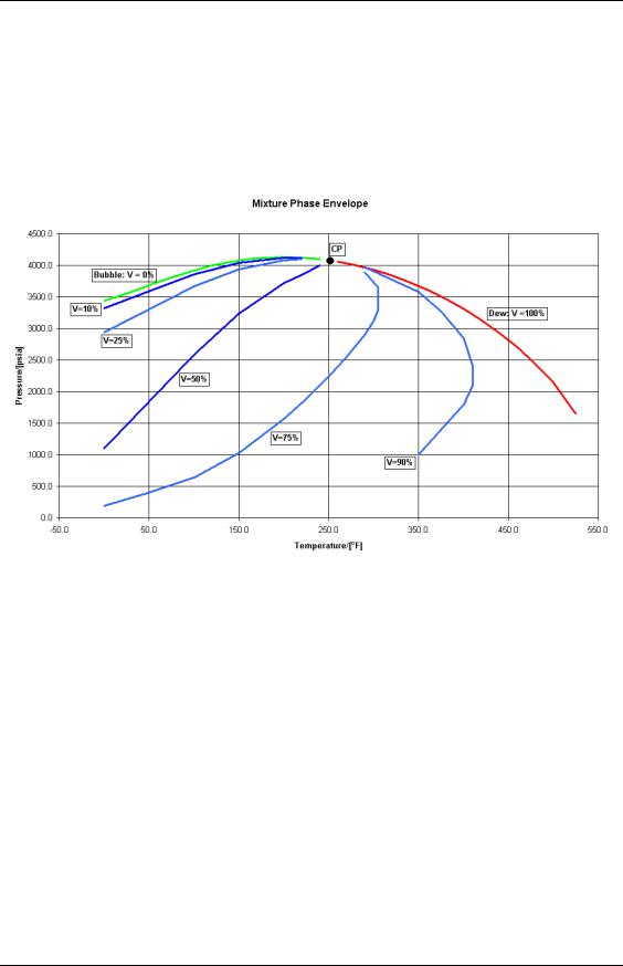
Adding more components to a mixture generally has the effect of broadening and raising the phase envelope. The extent of these changes depends primarily on the range of components in the mixture and their relative proportions [measured in moles – see section 5.1]. The phase envelope for a hypothetical mixture is shown below.

Figure 16: Multi-Component Phase Envelope.

In addition to the Bubble point line [vapour fraction, V = 0%] and Dew point line [V = 100 %], we have plotted lines of constants vapour fraction for V = 10, 25, 50,75 and 90%. All these lines, including the Bubble and Dew point lines converge at the critical point [approximately 4100 psia and 250 oF]. Using this plot, we can make sense of the five standard fluid types:

Dry Gas

Wet Gas

Gas Condensate

Volatile Oil

Crude Oil

We will discuss each of these fluid types by looking at relationship between reservoir temperature and phase envelope.

Roxar Oxford

27

12/12/12

PVT Analysis

3.3.1 Dry and Wet Gas

Although not marked explicitly, the Cricondentherm for this fluid is about Tcri 525 oF: it is highly unlikely a hydrocarbon reservoir would be found at such a temperature. For a lighter fluid mixture, the Tcrit will be lower and it is common to find Tres > Tcri.

If reservoir temperature is in excess of Tcri, under primary depletion where only pressure changes, at no point would the phase envelope be crossed: denoted 1 2 in the figure below. If surface conditions are at point 3d, still outside the two-phase region, the fluid is called Dry Gas.

Figure 17: Schematic Phase Envelope of a Dry and Wet Gas.

On the other hand, if surface conditions are at point 3w inside the two-phase region, then at some point in the production system liquid drop out will occur: this fluid is called Wet Gas.

As a rough guide, it has been suggested that any fluid which produces more than 50 Mscf/STB [ 8900 sm3/sm3] may be considered a wet gas. This corresponds to the Heptanes plus fraction being 1.0 mole percent or less. For most purposes, dry and wet gases can be modeled using correlations: this will be discussed further when we look at reduced properties and the Corresponding States theorem [see section 3.4].

3.3.2 Gas Condensates

Imagine the reservoir temperature for our multi-component mixture lies between Tcrit [approximately 252 oF] and Tcri. Further, assume the initial reservoir pressure is 4500 psia - we have a single-phase fluid.

Roxar Oxford

28

12/12/12

PVT Analysis

Under primary depletion, pressure can fall to about 3675 psia whereupon we find the dew point at which the first drop of liquid [heavier phase] appears from what we can now assume to be the vapour [lighter phase].

Figure 18: Liquid Dropout Profile from Gas Condensate [at constant composition]

As the pressure continues to fall, the liquid fraction builds to a peak of about 19% [by moles!] at about 3200 psia. As the pressure continues to fall, some of the dropped-out liquid re-vapourizes so that as we approach abandonment pressure around 1000 psia, the liquid fraction has fallen back to about 10%.

Note the behaviour just described is an idealized representation, which is only seen in the laboratory. Within a reservoir, the dropped-out liquid will generally remain immobile because of relative permeability effects [we will discuss this effect later in section 4.2.6]. The vapour however, will flow and therefore the fluid composition at a point will change with time.

The effect where a heavier liquid phase is evolved from a lighter vapour phase goes against our normal expectation of fluid behaviour under pressure reduction. Hence, the name Retrograde Condensation was termed: some authors still prefer to call Gas Condensates – Retrograde Gases.

As reservoir temperature approaches the critical temperature, we have already seen how the vapour fraction lines on the multi-component phase envelope are packing together. On the liquid dropout plot above, this would correspond to the slope of the curve becoming more nearly vertical and the maximum dropout approaching 50%. If the

Roxar Oxford

29

12/12/12

PVT Analysis

reservoir temperature is equal to the critical temperature, then as the pressure falls to equal the critical pressure, we immediately jump to a two-phase system [with 50% liquid and 50% vapour]. The two-phases will be identical and therefore indistinguishable.

Gas Condensates typically have GOR’s between 3.3 Mscf/STB [590 sm3/sm3] and 50 Mscf/STB [8900 sm3/sm3] although values up to 150 Mscf/STB have been reported. The stock tank oil derived from a gas condensate is usually lighter in colour than that derived from a crude oil. These rules are somewhat arbitrary. A more useful indicator is the mole fraction of the Heptanes-plus will be less than 12.5%.

3.3.3 Volatile Oils

If the reservoir temperature is less than the critical temperature, we get the expected fluid behaviour as pressure is reduced. An initially single-phase fluid, which we will subsequently label as liquid, on reaching the bubble point pressure yields a lighter vapour phase. The amount of vapour evolved depends on the proximity to the critical point. At temperatures just below the critical temperature, the amount of vapour produced approaches 50%. This vapour is rich in heavier hydrocarbons and will exhibit retrograde condensation as it’s produced. In some volatile oil reservoirs, it is common to find that half the produced stock tank oil entered the well bore as vapour. Because of this effect, the classical reservoir engineering material balance equations attributed to Schilthuis [see Dake, Chapter 3] will not work for a volatile oil.

GOR’s for volatile oils vary between 2.0 and 3.3 Mscf/STB. The Heptanes plus fraction varies between 12.5 and 20.0 mole percent. The liquid formation volume factor, denoted Bo [see section 4.2.5] will usually be greater than 2.0 RB/STB [2.0 m3/sm3].

3.3.4 Crude Oils

As the difference between reservoir temperature and critical temperature increases, with Tres < Tcrit, so the lines of constant vapour fraction spread out. Therefore, as pressure falls from the bubble point, the amount of vapour liberated falls. In addition, the liquid content of the liberated vapour is reduced. If the assumption that the liberated vapour can be treated as dry gas is acceptable, we can treat this fluid as a crude oil.

At pressures in excess of the bubble point, the crude will be referred to as being undersaturated, that is more vapour could be dissolved if it were present. At the bubble point, the crude is called saturated i.e. it holds as much vapour as it can. Strictly, at all pressures less than the bubble point pressure the liquid will be saturated, as vapour will continue to evolve.

Crude oils usually have GOR’s less than 2.0 Mscf/STB and their stock tank oil is often very dark in colour, usually black hence the alternative name of black oil. The Heptanes plus mole fraction will exceed 20%.

The relative simplicity of the crude oil phase behaviour has given rise to numerous correlations to describe their behaviour. These consist of expressions to calculate:

Roxar Oxford

30

12/12/12