pvt

PVT Analysis

something that doesn’t happen in the reservoir. The DLE or CVD are far more useful because they consider compositional changes and hence from the modeling point of view, are far more challenging.

4.2.4 Separator Test (SEP)

Well stream fluid arriving at surface is usually put through two or more stages of separation. A separator is effectively a large tank held at some pre-determined pressure and temperature, which allows the fluid to separate into vapour, liquid and optionally aqueous phases. Usually, the liquid from a first stage separator is taken to be the feed for the second stage, etc. Theoretically at least, the last stage is at standard conditions and the liquid arriving here is stock tank oil. In practice, especially in an offshore environment, the liquid will be put into a sales line at some pressure in excess of standard pressure. The vapour produced from each stage is collected together and reported as if it had been taken to standard conditions. Again, in practice, the vapour will rarely be taken down to standard conditions although the volumes are corrected to these conditions.

Figure 31: Schematic of 2-Stage Separator Test

The set of separator stages is some times referred to as a separator train. The train is an approximation to the processing plant used in practice. The key parameters to determine are the:

GOR at each stage and hence the total GOR

Roxar Oxford

51

12/12/12

PVT Analysis

Liquid Formation Volume Factor14 (FVF) and each stage and from Saturation pressure

Liquid and Vapour densities of liberated fluids at each stage.

The GOR is usually reported as the Gas Volume at standard conditions per Oil Volume at standard conditions [stock tank]. The volume of gas liberated at each stage, Vj, is at some elevated pressure and temperature (pj, Tj) at which its Z-factor, Zj, will be measured. Then, by the real gas law:

(4.4)

pV ZRT

See section 5.1.3. We can compute the volume that gas will occupy at standard conditions from:

		Z		T		p j
(4.5)	Vst	V j	st		st
			pst
						Z jTj

By definition, Zst = 1.0 and pst = 14.7 psia and Tst = 60 oF.

It is sometimes possible to adjust the pressure and temperature of the stages, generally the first stage pressure to maximize liquid production.

4.2.5 Differential Liberation (DLE)

This experiment is performed on crude oils and it begins by taking a known mass of the fluid to the bubble point pressure at reservoir temperature where the liquid volume is measured. Knowing the mass and volume, the density can be calculated. Then the pressure is reduced by a few 100 psia whereupon the liquid expands and some vapour is liberated. All the liberated vapour is removed from the cell. The vapour volume, moles, density and some times the composition are measured, as is the remaining oil volume. This process of expansion and extraction continues until the residual liquid is at a pressure of 1.0 atmosphere. The fluid is then cooled to standard temperature and the stock tank oil volume and density are measured.

The ratio of the liquid volume at each pressure point to that at standard conditions is reported as the Oil FVF, Bo. Summing the vapour volumes liberated between the current pressure and stock tank conditions and dividing that by the stock tank oil volume gives the Solution GOR, Rs.

14 Volume at stage conditions with respect to volume at stock tank conditions.

Roxar Oxford

52

12/12/12

PVT Analysis

Figure 32: Schematic of Differential Liberation Experiment.

Under certain conditions, the DLE can be seen as a tank-model of a crude oil reservoir. If when the pressure falls below the bubble point, either any liberated vapour is produced or it migrates upward to form or augment a gas cap, then we will always have a saturated liquid in the reservoir. The volumetric behaviour of that system is the DLE. However, the data from the DLE should NOT be used directly as the input to a black-oil reservoir simulation model. The DLE data must be corrected for the Flash Separation process that we approximate by the Separator Tests discussed in the previous section.

The equations commonly used for this conversion are:

				Bob
Rs Rsb (Rsdb			Rsd )
(4.xxx)				Bodb
	Bob
Bo Bod
	Bodb

Bob and Rsb are the bubble point oil FVF and solution GOR from the multi-stage separator flash. Bodb and Rsdb are the corresponding terms from the DLE. It should be noted that these equations are only an approximation. The recommended method is too flash the equilibrium oil from each stage of the DLE through the multi-stage separator system to give the true values of Bo and Rs. However, this process is time consuming and hence costly. An alternative approach using EoS modeling will be discussed in section 9.1.

Roxar Oxford

53

12/12/12

PVT Analysis

4.2.6 Constant Volume Depletion (CVD)

This experiment is performed on Gas Condensate and Volatile Oil fluids. Whether a DLE or a CVD is performed on a liquid sample depends on how much liquid remains at each stage. A near critical volatile oil would lose almost 50% of its fluid after its first stage of DLE: this may not leave enough fluid for analysis of subsequent stages.

As with the DLE, the experiment starts at the saturation pressure [liquid bubble point or vapour dew point] at which we note the fluid volume. This volume becomes the control volume for the experiment, denoted Vcell in the following figure.

Figure 33: Schematic of CVD Performed on Gas Condensate Fluid

As mentioned in section 4.2.2, the determination of the dew point pressure is a visual one. This may also be necessary for the volatile oil as the change in slope between the liquid and vapour plus liquid may not be clear since the liquid and vapour are so similar.

The CVD proceeds by reducing the pressure by several 100 psia say 500 – 700 psia. Then after allowing some time for the fluid to re-equilibrate, a volume of vapour is

removed such that the volume of vapour and liquid left in the cell is Vcell once more. The liquid volume in the cell is measured and reported as liquid drop-out:

(4.6)

Sliq Vliq Vcell

The number of moles of composition of that vapour.

vapour removed are measured as are the Z-factor and From the data reported, it is possible to back-compute the

Roxar Oxford

54

12/12/12

PVT Analysis

composition of the liquid remaining in the cell at each stage as shown below: see Whitson and Torp for details.

4.2.6.1 CVD Material Balance Check

Summarizing the CVD experiment once more, the data reported includes:

			Oil Samples Alternates
	Property		Property
T	Temperature
pd	Dew-point pressure	pb	Bubble-point pressure
Zd	Dew-point Z-factor	ob	Bubble-point density

As well as at each stage, k:

	Property
n	Moles removed
Z	Z-factor of removed gas
yi	Composition of removed gas
Sliq	Liquid saturation in the cell

Assuming we have 1.0 mole of fluid initially in place, the cell volume for a gas condensate sample is:

(4.xxx)	Vcell	Z (1) RT
		d
		pd

For a volatile oil sample, the cell volume is given by:

	(4.xxx)	V	cell		M ob
					ob

The bubble point mole weight, Mob, is calculated from:

	N
(4.xxx)	M ob zi(1) M i
	i 1

The initial feed composition, zi(1), is known as are the N-component mole weights, Mi. At stage k, the oil and gas volumes in the cell are:

Roxar Oxford

55

12/12/12

PVT Analysis

	(4.xxx)	Voil(k ) Vcell Sliq(k )
		Vgas(k ) Vcell (1	Sliq(k ) )

The total [subscript ‘t’] moles remaining in the cell at stage k is:

(4.xxx)

nt(k ) 1 n(k )

The moles of gas remaining in the cell at this stage is calculated from the Real Gas Law:

	(4.xxx)	ngas(k )		p(k )Vgas(k )
				Z (k ) RT

The moles of oil remaining is obtained by difference:

(4.xxx)

noil(k ) nt(k ) ngas(k )

The overall composition of the mixture in the cell at stage k is obtained by summing up the moles of vapour removed to date:

		k	yi( j)
(4.xxx)	nt(k ) zi(k ) zi(1)	n( j) n( j 1)
		j 2

The composition of the oil remaining in the cell at stage k is then obtained from:

(4.xxx)

noil(k ) xi(k ) ngas(k ) yi(k )

nt(k ) zi(k )

With these estimated liquid compositions and the measured vapour compositions, we can calculate K-values using (4.1). If these K-values are plotted as a function of pressure, we expect to see certain trends. In particular, the K-values should plot in order of decreasing volatility [increasing mole weight], they should not cross and they should converge as pressure increases.

Knowing the oil and gas compositions, we can calculate the respective phase mole weights and hence their masses given the phase moles. With the phase volumes and masses, we can calculate the phase densities. This whole procedure is ideal spreadsheet material!

In practice, hardly any of the CVD’s generated before the 1980’s satisfied the conditions above. However, since then, most of the service laboratories have got wise to the analysis technique of Whitson and Torp and they massage the data. Whilst this may be a valid and useful data check, it is still nice to see the original data also.

In conjunction with the Standing K-values, see section 4.1.4, the data from the CVD can be used to estimate stock tank gas and oil yields.

4.2.7 Other Experiments

A number of other experiments are performed under special circumstances: these are all usually connected with the possibility of gas injection or gas re-cycling.

Roxar Oxford

56

12/12/12

PVT Analysis

The most simple of these tests is the Swelling Test. Here, volumes [or moles] of a specified composition gas are added to the reservoir fluid in a number of stages. Prior to and after each addition, the fluid is taken to its saturation pressure. The relative change in volume is the swelling factor. This is reported in addition to the series of saturation pressures. If applied to an original liquid, there will be some cumulative vapour volume, which will result in a vapour mixture; i.e. bubble-points become dew points.

Figure 34: Schematic of the Swelling Test.

A variant on the Swelling Test is the Vapourisation Test. Here, the original fluid is initialised at some pressure less than the saturation pressure and the volume is noted. A volume of gas is added the mixture is allowed to equilibrate and enough fluid [vapour] is removed to return the mixture volume to the volume previously noted. Here, the idea is to test how an injection gas might vapourise heavy ends from a dropped-out liquid phase as it passes over reservoir liquid.

A third gas injection test is the Slim Tube experiment. Here a long length of narrow bore tubing, say 10 m by 6 mm, is packed with porous material, usually sand. The tube is filled with reservoir fluid and the pressure is set. Gas injection then starts at one end and the produced fluid is monitored at the other end. The volume of oil produced as a percentage of the total production is then plotted against pressure. By definition, the

Minimum Miscibility Pressure (MMP) is defined as Recovery of 90% of the Original Oil In Place (OOIP) displaced by the injection of 1.2 Pore Volumes Injected (PVI) of injection gas. Recovery is defined as being:

Roxar Oxford

57

12/12/12

PVT Analysis

(Volume of oil at stock tank condition)/(original volume of slim tube at pressure P).

Figure 35: Schematic of the Slim Tube Apparatus [ref. See Figure 27].

A near 100% recovery is achieved when the injection gas and reservoir fluid mixture is always single-phase at the pressure of interest. The MMP is the lowest pressure at which these two fluids will be single-phase for all possible blends of the two fluids.

Roxar Oxford

58

12/12/12

PVT Analysis

5.Equations of State

In order to predict how a fluid mixture of given composition behaves at given conditions of pressure and temperature, we invoke various thermodynamic models.

5.1 Development of the Ideal Gas Law

The three principle contributions to the development of the Ideal Gas Law were from Boyle (1662), Charles (1787) and Avogadro (1811).

Boyle conducted experiments on simple gases and observed that [at constant temperature]; the volume of the gas was inversely proportional to its pressure, namely:

(5.1)	V	1	.
		p

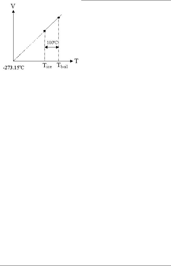
Charles observed that [at constant pressure], the volume of a gas is directly proportional to its temperature, namely:

(5.2)

V T .

This observation was used as a mechanism to define temperature. At a pressure of 1 atmosphere, it was decided to have 100 units separate the ice and steam points of pure water – the Celsius scale. However, the implication of this definition is there is a zerotemperature limit at which the volume of a gas becomes zero: this demonstrates one of the limitations of this model, which will be discussed in the next section.

Figure 36: Charles’ Law Behaviour for Water Implying Zero Temperature.

Roxar Oxford

59

12/12/12

PVT Analysis

By the time Avogadro performed his series of experiments, the elemental nature of matter was being recognized. Avogadro observed that for a gas [at constant pressure and temperature], the volume is directly proportional to the number of elements, namely:

(5.3)

V n .

Avagadro’s hypothesis has profound implications. Equal volumes of two different gases at the same [low, near-atmospheric] pressure and [normal] temperature must contain the same number of elements or molecules. Therefore, the ratio of weight of the two gases must be the ratio of the weight of the molecules. Given a suitable reference, we now have a method by which we can define the molecular weight, or mole weight for short, of a given chemical species.

5.1.1 The Mole

In particular, Mw grams of [an ideal] gas at 1 atmosphere pressure and 15 oC contains 1 gram-mole of gas and occupies a volume of 22.4x10-3 m3: Mw is the mole weight which for the diatomic molecules of hydrogen, nitrogen and oxygen are 2.0, 14.0 and 16.0, respectively. In field units, 1 lbmole of gas, weighing Mw lb., occupies 379.4 ft3 at 14.7 psia and 60 oF.

The use of the correct mass-basis when considering moles is most important. Combining the three relationships above, we have:

(5.4)	pV nT
Or:
(5.5)	pV nRT

Where R is called the universal gas constant, or gas constant for short, and whose numerical value depends on the units for p, V, n and T.

In field units with p in psia, V in ft3, n in lbmoles and T in degrees Rankine: R = 10.732 [psia.ft3/(lbmole.oR],

Whereas in oilfield-metric units with p in bars, V in m3, n in kgmoles and T in Kelvin: R = 0.08314 [bars.m3/(kgmole. K)].

If we consider 1 mole of material [in the appropriate mass units], we can write the Ideal Gas Law as:

(5.6)

pVm RT

Where the subscript m denotes a molar quantity, in this case the molar volume.

Moles are an extremely powerful tool in fluid modeling. of molecules, or alternatively the mass of material,

Because they tell us the number they are subject to the usual

Roxar Oxford

60

12/12/12