pvt

PVT Analysis

4.1.4.4 Checking the Data

A number of analysis techniques can be employed to ensure any recombined sample is representative. Firstly, when the liquid bottle is opened back in the laboratory, the bubble point pressure should be the same as the separator pressure at which it was sampled, corrected for temperature12. Secondly, since we have a vapour and liquid composition,

then we know the vapour and liquid mole fractions of all components, denoted yi , xi , respectively. From the gas and oil composition’s we can calculate the K-values:

y

(4.1) Ki xi

i

Standing suggested that these measured K-values should obey:

(4.2)

log10 Ki psep A0 A1Fi

The Fi are given by:

1 Tbi 1 T

pci

(4.3)

Fi

log

1 T

1 T

p

bi

ci

sc

T ,T

, p

ci

are

the

ith components’ normal boiling point temperature, critical

bi ci

temperature and critical pressure and psc is standard pressure in a consistent unit set. The constants (A0, A1) are calculated from:

	A	1.200	4.5 10 4 p	sep	15.0	10 8	p2
(4.4)	0						sep
	A	0.890	1.7 10 4 p		3.5	10 8	p2
				sep
	1						sep

The separator pressure must be measured in psia. Equation (4.2) is generally assumed

valid for hydrocarbon mixtures at pressures up to 1000 psia and temperatures up to 200 oF.

4.1.4.5 Recombination Example

The well stream fluid is flashed via the test separator into gas and oil samples. The samples are collected in bottles and sent to the laboratory. The gas and oil flow rates from the test separator are noted to give a gas-oil-ratio for the subsequent recombination calculation. The gas sample is sent straight to compositional analysis via the gas chromatogram. The oil sample is flashed at ambient or Stock Tank Conditions (STC) with the stock streams then being analysed by gas chromatogram: again, the gas and oil volumes are noted to give the ST flash GOR.

The surface separation process can be illustrated in the following schematic.

12 As a rule, bubble-point pressure of separator liquid samples increase between 3 and 4 psia per degree Fahrenheit.

Roxar Oxford

41

12/12/12

PVT Analysis

Figure 22: Surface Separator Analysis.

The typical data looks like the following Excel chart: compositions, GOR’s, etc. taken from Table 2.15 of Pedersen et al.

The input data is highlighted in the bordered cells. This includes the stock tank oil and gas compositions, the separator gas composition, the stock tank oil plus fraction mole weight and stock tank oil density, the separator and ambient GOR’s and the separator FVF. The calculated reservoir composition is shown in the final column of the sheet.

The basis of the calculation is the assumption of 1.0 STB of stock tank oil. Given a density in lb/ft3, this is converted to lb./STB by multiplying by 5.615 ft3/STB. The stocktank oil mole-weight is calculated via Equation 5.9 with the user-supplied value of plus fraction mole weight.

The moles of oil in 1.0 STB can now be calculated from the density [in lb./STB] divided by the mole weight.

The quoted separator GOR is the produced gas at standard conditions, per barrel of oil at separator conditions. To convert the separator GOR to oil at standard conditions, multiply by the separator oil FVF. Now since both GOR’s are quoted per stock tank barrel, we can assume the stated volumes of gas are to be added to our 1.0 STB. Standard volumes of gas can be converted directly to moles by dividing by 379.4 [scf/lbmole]. We can add the moles of stock tank oil, stock tank gas and separator gas directly. The stream mole fractions are just stream moles per total moles. Finally, we multiply the stream mole fractions by the stream compositions and add to yield the reservoir fluid composition. A similar calculation involving just the stock tank oil and gas streams will back calculate the pre-flashed separator oil composition.

Roxar Oxford

42

12/12/12

PVT Analysis

Recombine Test Separator Streams to Calculate Reservoir Composition

Comp	Mw	ST Oil	Mw	ST Gas	Mw	Sep Gas	Mw
N2	28.0	0.00	0.0	0.20	5.6	0.66	18.5
CO2	44.0	0.00	0.0	3.96	174.2	5.65	248.6
C1	16.0	0.00	0.0	24.85	397.6	68.81	1101.0
C2	30.0	0.20	6.0	20.40	612.0	12.86	385.8
C3	44.0	2.14	94.2	28.41	1250.0	7.94	349.4
iC4	58.0	1.10	63.8	4.78	277.2	0.94	54.5
nC4	58.0	4.25	246.5	10.97	636.3	1.96	113.7
iC5	72.0	2.68	193.0	2.21	159.1	0.34	24.5
nC5	72.0	4.32	311.0	2.53	182.2	0.42	30.2
C6	96.0	6.66	639.4	1.05	100.8	0.22	21.1
C7	110.0	11.90	1309.0	0.54	59.4	0.15	16.5
C8	124.0	13.14	1629.4	0.10	12.4	0.05	6.2
C9	138.0	7.73	1066.7	0.00	0.0	0.00	0.0
C10+	228.5	45.88	10483.6	0.00	0.0	0.00	0.0
Sums		100.00	160.4	100.00	38.7	100.00	23.7
Dens	(lb/ft3)
		53.69
	(lb/stb)	301.47
	Separator GOR			scf/bbl
			2482		Separator GOR(*)		2891.53 scf/stb
	Separator FVF		1.165	bbl/stb
	Ambient GOR		207	scf/stb
		ST Oil		ST Gas		Sep Gas		Total
Moles		1.8792		0.5456		7.6213		10.0461
Mol%		0.1871		0.0543		0.7586
Comp		ST Oil	Mol	ST Gas	Mol	Sep Gas	Mol	Res Fluid
N2		0.00	0.00	0.20	0.01	0.66	0.50
								0.51
CO2		0.00	0.00	3.96	0.22	5.65	4.29	4.50
C1		0.00	0.00	24.85	1.35	68.81	52.20	53.55
C2		0.20	0.04	20.40	1.11	12.86	9.76	10.90
C3		2.14	0.40	28.41	1.54	7.94	6.02	7.97
iC4		1.10	0.21	4.78	0.26	0.94	0.71	1.18
nC4		4.25	0.79	10.97	0.60	1.96	1.49	2.88
iC5		2.68	0.50	2.21	0.12	0.34	0.26	0.88
nC5		4.32	0.81	2.53	0.14	0.42	0.32	1.26
C6		6.66	1.25	1.05	0.06	0.22	0.17	1.47
C7		11.90	2.23	0.54	0.03	0.15	0.11	2.37
C8		13.14	2.46	0.10	0.01	0.05	0.04	2.50
C9		7.73	1.45	0.00	0.00	0.00	0.00	1.45
C10+		45.88	8.58	0.00	0.00	0.00	0.00	8.58
Sums		100.00	18.71	100.00	5.43	100.00	75.86
								100.00

Roxar Oxford

43

12/12/12

PVT Analysis

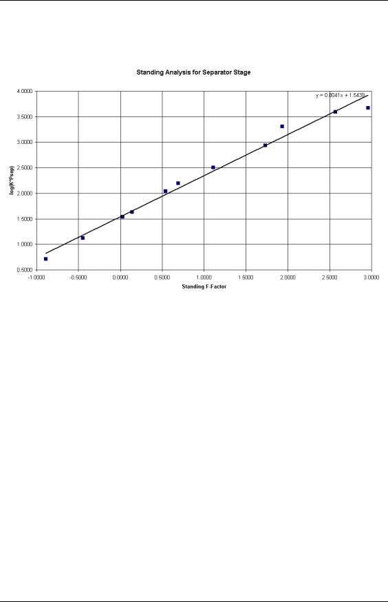
Using the Standing procedure discussed in the previous section, we can generate the following plot:

Figure 23: Standing Analysis for the Separator Stage.

There is some scatter of the points, especially for high F-factors, which correspond to the more volatile species. However, this particular analysis would be regarded as satisfactory.

Roxar Oxford

44

12/12/12

PVT Analysis

4.2 Laboratory Analysis

Having obtained what are hoped to be one or more representative samples, the next task is to analyse them. Here the first task is to perform a compositional determination to find which components are present and in what proportions. Then a set of standard experiments should be performed to determine a set of important parameters. The parameters measured depend on the nature of the fluid, i.e. reservoir liquid or vapour.

4.2.1 Compositional Determination

The workhorse in this area is the gas chromatogram. A gas chromatogram usually comes in one of two types, Packed or Capillary columns. The packed column consists of a glass or stainless steel coil, typically 1-5 m in length and 5 mm inner diameter. The capillary columns are thin fused silica, typically 10-100 m in length with an inner diameter of 250m.

Figure 24: Schematic of a GC System.

The sample is injected into the column, which is housed in a temperature-controlled oven. As the temperature is increased on some pre-programmed schedule, the components will boil depending on their volatility. An inert carrier gas such as helium or argon then carries the components along the tube to a detector. The most popular types of detector are the Flame Ionization Detector (FID) and the Thermal Conductivity Detector (TCD).

The effluent from the GC mixes with the air/hydrogen mixture and passes through a flame. The resulting ions are collected between the electrodes to produce an electrical signal. The FID is very sensitive but it destroys the sample.

The TCD consists of an electrically heated wire whose resistance is effected by the thermal conductivity of the surrounding gas. The change in resistance can be correlated to the nature of the surrounding gas. The TCD is not as accurate as the FID but it is nondestructive.

Roxar Oxford

45

12/12/12

PVT Analysis

Figure 25: Schematic of the FID [from www.scimedia.com].

Liquid samples can be analysed up to C10+ using the same capillary column technique. If a breakdown of the C10+ fraction into C10, , C19, C20+ is required, mini distillation is required. The C10+ residue is heated at reduced pressure, to prevent thermal cracking, in a series of boiling point increments corresponding to those which define the Single Carbon Number groups, see section 2.7.

In a detailed study by Eyton, the repeatability and hence the accuracy of compositional measurements was evaluated. Eyton concluded that given a mole percentage of xi, the error bands would be:

(4.xxx)

xi

0.07xi0.43

Thus as the mole percentage of a component approaches 100.0%, the measurement error can be assumed to be 0.5% whereas if the mole percent is as low as 0.01%, the measurement error is of the same order.

Regardless of the technique employed, a residue or plus fraction will be left: see section 2.8. The density or specific gravity of the plus fraction should measured relatively accurately. The measurement of molecular weight is a lot more difficult and therefore prone to error. The most common technique is freezing point depression where a small amount of the plus fraction is added to a pure solvent such as benzene. The freezing point of the mixture will be depressed by some T, the value of which depends on the mole weight of the contaminant.

Roxar Oxford

46

12/12/12

PVT Analysis

Figure 26: Freezing point depression diagram [from Pedersen et al.]

The apparatus must be calibrated with great care using substances of known molecular weight. Similarly, the solvent must be of the highest purity. Errors of 10% are common.

4.2.2 Saturation Pressure (SAT)

The bubble point pressure for a reservoir liquid or the dew point pressure for a reservoir vapour is one of the important measurements performed. The exact mechanics of the measurement depend on the fluid type but in both cases it begins by loading a volume of the reservoir fluid into a PVT cell. This cell is placed in chamber whose temperature can be set to the reservoir temperature. Pistons can raise and lower the pressure and valves allow fluid to be injected and removed from the top and bottom of the cell. Some cells contain a window, located towards the bottom of the cell to allow visual inspection of the contents.

4.2.2.1 The PVT Cell

Below is a schematic representation of a Gas Condensate PVT cell. The solid black line surrounding the cell indicates the oven in which reservoir temperature can be simulated. The proportional mercury pumps allow the reservoir fluid to be pushed from above and below to allow the gas/oil interface to be located centrally where the cell contracts. A mica window allows a camera too see into the cell via a fibre optic cable. A stirring device is added to speed-up the equilibration process.

Roxar Oxford

47

12/12/12

PVT Analysis

Figure 27: Schematic of a Gas Condensate PVT cell13

For a liquid, the pressure is raised to some high pressure, generally slightly in excess of initial reservoir pressure. Then, the pressure is reduced in a series of stages, noting the volume of the fluid at each stage. If a plot of volume versus pressure is made, the behaviour on the following plot is observed.

Figure 28: Change in Slope of p-V curve around the Bubble Point.

13 See Heriot-Watt Petroleum Engineering web pages: http://www.pet.hw.ac.uk/3frame.html.

Roxar Oxford

48

12/12/12

PVT Analysis

In particular, note the change in slope – this identifies the bubble point pressure since at pressures less than 3900 psia, the higher slope shows the presence of a more compressible system i.e. liquid and vapour.

This fluid was subsequently labeled a volatile oil and the change in slope is still evident. However, for very near critical liquids, this technique may not be sensitive enough and the technique used for gas condensates may be required.

The evolution of a liquid from a vapour will not produce any significant change in slope on the p-V plot like the one seen above: instead, a visual determination is required. Because of the hostile conditions, remote visual observation is made of the cell using a fibre optic cable. As pressure is reduced, a careful watch is made for the point when the first drop of dew [liquid] is seen.

This measurement is prone to error. There is considerable debate as to how long the cell should be left after each pressure reduction step before the observation is made: this is because equilibrium is not instantaneous. Various stirring or mixing techniques are used to try to speed up the process. Contamination such as grease on the seals and o-rings may cause early liquid formation. Finally, small droplets of liquid, which appear in the top of the cell, may not trickle down to the bottom of cell where the observation is usually made.

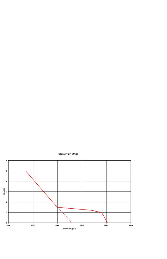
Some condensate samples exhibit an effect called the liquid dropout tail. This is where a small but apparently measurable liquid saturation may exist. On the following figure, the dew point pressure predicted by extrapolating the main trend to zero would suggest pdew 5300 psia whereas the measured value is in excess of 6000 psia: discrepancies of over 1000 psia have been seen. Nevertheless, the liquid drop-out in these “tails” is generally less than 2% therefore we have to ask ourselves whether ignoring it will have a significant effect on the way we model and develop the fluid – probably not.

Figure 29: Liquid Dropout “Tail” Shown by Some Gas Condensates

Roxar Oxford

49

12/12/12

PVT Analysis

4.2.3 Constant Composition Expansion (CCE)

The CCE, some times called the Constant Mass Experiment (CME), is the experiment during which the saturation pressure is determined. The fluid-containing cell is heated in an oven to reservoir temperature and pressured up to some pressure in excess of initial reservoir pressure: the fluid volume is measured. Since this initial pressure is presumably single-phase, either the liquid density or vapour Z-factor are determined depending on the nature of the single-phase fluid. These measurements are repeated for all single-phase states, including the saturation pressure.

The pressure is reduced in a number of stages down to some low pressure, typically 1000 to 2000 psia: no fluid is ever removed from the cell, hence the name Constant Composition Expansion. The density of pressure points is increased either side of the saturation pressure, otherwise increments of between 500 psia to 700 psia are generally used: at each pressure point, the fluid volume is measured. Rather than quoting the absolute volumes, the laboratory will quote the volume relative to that at the saturation pressure – the [Total] Relative Volume. For gas condensate systems, it is usual to measure the liquid dropout measured as the liquid volume relative to the total fluid volume at the dew point pressure.

Figure 30: Schematic of CCE applied to Gas Condensate Fluid.

The main aim of the CCE is as the vehicle to find the saturation pressure. Measurements made above the saturation pressure of density or Z-factor and viscosity are useful. Relative volume and liquid dropout measurements at pressures less than saturation pressure are of limited value because of the constant composition assumption –

Roxar Oxford

50

12/12/12