

- •CONTENTS
- •Preface
- •Contributors
- •1 Introduction to Toxicology
- •1.1 Definition and Scope, Relationship to Other Sciences, and History
- •1.1.2 Relationship to Other Sciences
- •1.1.3 A Brief History of Toxicology
- •1.3 Sources of Toxic Compounds
- •1.3.1 Exposure Classes
- •1.3.2 Use Classes
- •1.4 Movement of Toxicants in the Environment
- •Suggested Reading
- •2.1 Introduction
- •2.2 Cell Culture Techniques
- •2.2.1 Suspension Cell Culture
- •2.2.2 Monolayer Cell Culture
- •2.2.3 Indicators of Toxicity in Cultured Cells
- •2.3 Molecular Techniques
- •2.3.1 Molecular Cloning
- •2.3.2 cDNA and Genomic Libraries
- •2.3.3 Northern and Southern Blot Analyses
- •2.3.4 Polymerase Chain Reaction (PCR)
- •2.3.5 Evaluation of Gene Expression, Regulation, and Function
- •2.4 Immunochemical Techniques
- •Suggested Reading
- •3.1 Introduction
- •3.2 General Policies Related to Analytical Laboratories
- •3.2.1 Standard Operating Procedures (SOPs)
- •3.2.2 QA/QC Manuals
- •3.2.3 Procedural Manuals
- •3.2.4 Analytical Methods Files
- •3.2.5 Laboratory Information Management System (LIMS)
- •3.3 Analytical Measurement System
- •3.3.1 Analytical Instrument Calibration
- •3.3.2 Quantitation Approaches and Techniques
- •3.4 Quality Assurance (QA) Procedures
- •3.5 Quality Control (QC) Procedures
- •3.6 Summary
- •Suggested Reading
- •4 Exposure Classes, Toxicants in Air, Water, Soil, Domestic and Occupational Settings
- •4.1 Air Pollutants
- •4.1.1 History
- •4.1.2 Types of Air Pollutants
- •4.1.3 Sources of Air Pollutants
- •4.1.4 Examples of Air Pollutants
- •4.1.5 Environmental Effects
- •4.2 Water and Soil Pollutants
- •4.2.1 Sources of Water and Soil Pollutants
- •4.2.2 Examples of Pollutants
- •4.3 Occupational Toxicants
- •4.3.1 Regulation of Exposure Levels
- •4.3.2 Routes of Exposure
- •4.3.3 Examples of Industrial Toxicants
- •Suggested Reading
- •5 Classes of Toxicants: Use Classes
- •5.1 Introduction
- •5.2 Metals
- •5.2.1 History
- •5.2.2 Common Toxic Mechanisms and Sites of Action
- •5.2.3 Lead
- •5.2.4 Mercury
- •5.2.5 Cadmium
- •5.2.6 Chromium
- •5.2.7 Arsenic
- •5.2.8 Treatment of Metal Poisoning
- •5.3 Agricultural Chemicals (Pesticides)
- •5.3.1 Introduction
- •5.3.3 Organochlorine Insecticides
- •5.3.4 Organophosphorus Insecticides
- •5.3.5 Carbamate Insecticides
- •5.3.6 Botanical Insecticides
- •5.3.7 Pyrethroid Insecticides
- •5.3.8 New Insecticide Classes
- •5.3.9 Herbicides
- •5.3.10 Fungicides
- •5.3.11 Rodenticides
- •5.3.12 Fumigants
- •5.3.13 Conclusions
- •5.4 Food Additives and Contaminants
- •5.5 Toxins
- •5.5.1 History
- •5.5.2 Microbial Toxins
- •5.5.3 Mycotoxins
- •5.5.4 Algal Toxins
- •5.5.5 Plant Toxins
- •5.5.6 Animal Toxins
- •5.6 Solvents
- •5.7 Therapeutic Drugs
- •5.8 Drugs of Abuse
- •5.9 Combustion Products
- •5.10 Cosmetics
- •Suggested Reading
- •6 Absorption and Distribution of Toxicants
- •6.1 Introduction
- •6.2 Cell Membranes
- •6.3 Mechanisms of Transport
- •6.3.1 Passive Diffusion
- •6.4 Physicochemical Properties Relevant to Diffusion
- •6.4.1 Ionization
- •6.5 Routes of Absorption
- •6.5.1 Extent of Absorption
- •6.5.2 Gastrointestinal Absorption
- •6.5.3 Dermal Absorption
- •6.5.4 Respiratory Penetration
- •6.6 Toxicant Distribution
- •6.6.1 Physicochemical Properties and Protein Binding
- •6.7 Toxicokinetics
- •Suggested Reading
- •7 Metabolism of Toxicants
- •7.1 Introduction
- •7.2 Phase I Reactions
- •7.2.4 Nonmicrosomal Oxidations
- •7.2.5 Cooxidation by Cyclooxygenases
- •7.2.6 Reduction Reactions
- •7.2.7 Hydrolysis
- •7.2.8 Epoxide Hydration
- •7.2.9 DDT Dehydrochlorinase
- •7.3 Phase II Reactions
- •7.3.1 Glucuronide Conjugation
- •7.3.2 Glucoside Conjugation
- •7.3.3 Sulfate Conjugation
- •7.3.4 Methyltransferases
- •7.3.7 Acylation
- •7.3.8 Phosphate Conjugation
- •Suggested Reading
- •8 Reactive Metabolites
- •8.1 Introduction
- •8.2 Activation Enzymes
- •8.3 Nature and Stability of Reactive Metabolites
- •8.4 Fate of Reactive Metabolites
- •8.4.1 Binding to Cellular Macromolecules
- •8.4.2 Lipid Peroxidation
- •8.4.3 Trapping and Removal: Role of Glutathione
- •8.5 Factors Affecting Toxicity of Reactive Metabolites
- •8.5.1 Levels of Activating Enzymes
- •8.5.2 Levels of Conjugating Enzymes
- •8.5.3 Levels of Cofactors or Conjugating Chemicals
- •8.6 Examples of Activating Reactions
- •8.6.1 Parathion
- •8.6.2 Vinyl Chloride
- •8.6.3 Methanol
- •8.6.5 Carbon Tetrachloride
- •8.6.8 Acetaminophen
- •8.6.9 Cycasin
- •8.7 Future Developments
- •Suggested Reading
- •9.1 Introduction
- •9.2 Nutritional Effects
- •9.2.1 Protein
- •9.2.2 Carbohydrates
- •9.2.3 Lipids
- •9.2.4 Micronutrients
- •9.2.5 Starvation and Dehydration
- •9.2.6 Nutritional Requirements in Xenobiotic Metabolism
- •9.3 Physiological Effects
- •9.3.1 Development
- •9.3.2 Gender Differences
- •9.3.3 Hormones
- •9.3.4 Pregnancy
- •9.3.5 Disease
- •9.3.6 Diurnal Rhythms
- •9.4 Comparative and Genetic Effects
- •9.4.1 Variations Among Taxonomic Groups
- •9.4.2 Selectivity
- •9.4.3 Genetic Differences
- •9.5 Chemical Effects
- •9.5.1 Inhibition
- •9.5.2 Induction
- •9.5.3 Biphasic Effects: Inhibition and Induction
- •9.6 Environmental Effects
- •9.7 General Summary and Conclusions
- •Suggested Reading
- •10 Elimination of Toxicants
- •10.1 Introduction
- •10.2 Transport
- •10.3 Renal Elimination
- •10.4 Hepatic Elimination
- •10.4.2 Active Transporters of the Bile Canaliculus
- •10.5 Respiratory Elimination
- •10.6 Conclusion
- •Suggested Reading
- •11 Acute Toxicity
- •11.1 Introduction
- •11.2 Acute Exposure and Effect
- •11.3 Dose-response Relationships
- •11.4 Nonconventional Dose-response Relationships
- •11.5 Mechanisms of Acute Toxicity
- •11.5.1 Narcosis
- •11.5.2 Acetylcholinesterase Inhibition
- •11.5.3 Ion Channel Modulators
- •11.5.4 Inhibitors of Cellular Respiration
- •Suggested Reading
- •12 Chemical Carcinogenesis
- •12.1 General Aspects of Cancer
- •12.2 Human Cancer
- •12.2.1 Causes, Incidence, and Mortality Rates of Human Cancer
- •12.2.2 Known Human Carcinogens
- •12.3 Classes of Agents Associated with Carcinogenesis
- •12.3.2 Epigenetic Agents
- •12.4 General Aspects of Chemical Carcinogenesis
- •12.5 Initiation-Promotion Model for Chemical Carcinogenesis
- •12.6 Metabolic Activation of Chemical Carcinogens and DNA Adduct Formation
- •12.7 Oncogenes
- •12.8 Tumor Suppressor Genes
- •12.8.1 Inactivation of Tumor Suppressor Genes
- •12.8.2 p53 Tumor Suppressor Gene
- •12.9 General Aspects of Mutagenicity
- •12.10 Usefulness and Limitations of Mutagenicity Assays for the Identification of Carcinogens
- •Suggested Reading
- •13 Teratogenesis
- •13.1 Introduction
- •13.2 Principles of Teratology
- •13.3 Mammalian Embryology Overview
- •13.4 Critical Periods
- •13.5 Historical Teratogens
- •13.5.1 Thalidomide
- •13.5.2 Accutane (Isotetrinoin)
- •13.5.3 Diethylstilbestrol (DES)
- •13.5.4 Alcohol
- •13.6 Testing Protocols
- •13.6.1 FDA Guidelines for Reproduction Studies for Safety Evaluation of Drugs for Human Use
- •13.6.3 Alternative Test Methods
- •13.7 Conclusions
- •Suggested Reading
- •14 Hepatotoxicity
- •14.1 Introduction
- •14.1.1 Liver Structure
- •14.1.2 Liver Function
- •14.2 Susceptibility of the Liver
- •14.3 Types of Liver Injury
- •14.3.1 Fatty Liver
- •14.3.2 Necrosis
- •14.3.3 Apoptosis
- •14.3.4 Cholestasis
- •14.3.5 Cirrhosis
- •14.3.6 Hepatitis
- •14.3.7 Oxidative Stress
- •14.3.8 Carcinogenesis
- •14.4 Mechanisms of Hepatotoxicity
- •14.5 Examples of Hepatotoxicants
- •14.5.1 Carbon Tetrachloride
- •14.5.2 Ethanol
- •14.5.3 Bromobenzene
- •14.5.4 Acetaminophen
- •14.6 Metabolic Activation of Hepatotoxicants
- •Suggested Reading
- •15 Nephrotoxicity
- •15.1 Introduction
- •15.1.1 Structure of the Renal System
- •15.1.2 Function of the Renal System
- •15.2 Susceptibility of the Renal System
- •15.3 Examples of Nephrotoxicants
- •15.3.1 Metals
- •15.3.2 Aminoglycosides
- •15.3.3 Amphotericin B
- •15.3.4 Chloroform
- •15.3.5 Hexachlorobutadiene
- •Suggested Reading
- •16 Toxicology of the Nervous System
- •16.1 Introduction
- •16.2 The Nervous system
- •16.2.1 The Neuron
- •16.2.2 Neurotransmitters and their Receptors
- •16.2.3 Glial Cells
- •16.3 Toxicant Effects on the Nervous System
- •16.3.1 Structural Effects of Toxicants on Neurons
- •16.3.2 Effects of Toxicants on Other Cells
- •16.4 Neurotoxicity Testing
- •16.4.1 In vivo Tests of Human Exposure
- •16.4.2 In vivo Tests of Animal Exposure
- •16.4.3 In vitro Neurochemical and Histopathological End Points
- •16.5 Summary
- •Suggested Reading
- •17 Endocrine System
- •17.1 Introduction
- •17.2 Endocrine System
- •17.2.1 Nuclear Receptors
- •17.3 Endocrine Disruption
- •17.3.1 Hormone Receptor Agonists
- •17.3.2 Hormone Receptor Antagonists
- •17.3.3 Organizational versus Activational Effects of Endocrine Toxicants
- •17.3.4 Inhibitors of Hormone Synthesis
- •17.3.5 Inducers of Hormone Clearance
- •17.3.6 Hormone Displacement from Binding Proteins
- •17.4 Incidents of Endocrine Toxicity
- •17.4.1 Organizational Toxicity
- •17.4.2 Activational Toxicity
- •17.4.3 Hypothyroidism
- •17.5 Conclusion
- •Suggested Reading
- •18 Respiratory Toxicity
- •18.1 Introduction
- •18.1.1 Anatomy
- •18.1.2 Cell Types
- •18.1.3 Function
- •18.2 Susceptibility of the Respiratory System
- •18.2.1 Nasal
- •18.2.2 Lung
- •18.3 Types of Toxic Response
- •18.3.1 Irritation
- •18.3.2 Cell Necrosis
- •18.3.3 Fibrosis
- •18.3.4 Emphysema
- •18.3.5 Allergic Responses
- •18.3.6 Cancer
- •18.3.7 Mediators of Toxic Responses
- •18.4 Examples of Lung Toxicants Requiring Activation
- •18.4.1 Introduction
- •18.4.2 Monocrotaline
- •18.4.3 Ipomeanol
- •18.4.4 Paraquat
- •18.5 Defense Mechanisms
- •Suggested Reading
- •19 Immunotoxicity
- •19.1 Introduction
- •19.2 The Immune System
- •19.3 Immune Suppression
- •19.4 Classification of Immune-Mediated Injury (Hypersensitivity)
- •19.5 Effects of Chemicals on Allergic Disease
- •19.5.1 Allergic Contact Dermatitis
- •19.5.2 Respiratory Allergens
- •19.5.3 Adjuvants
- •19.6 Emerging Issues: Food Allergies, Autoimmunity, and the Developing Immune System
- •Suggested Reading
- •20 Reproductive System
- •20.1 Introduction
- •20.2 Male Reproductive Physiology
- •20.3 Mechanisms and Targets of Male Reproductive Toxicants
- •20.3.1 General Mechanisms
- •20.3.2 Effects on Germ Cells
- •20.3.3 Effects on Spermatogenesis and Sperm Quality
- •20.3.4 Effects on Sexual Behavior
- •20.3.5 Effects on Endocrine Function
- •20.4 Female Reproductive Physiology
- •20.5 Mechanisms and Targets of Female Reproductive Toxicants
- •20.5.1 Tranquilizers, Narcotics, and Social Drugs
- •20.5.2 Endocrine Disruptors (EDs)
- •20.5.3 Effects on Germ Cells
- •20.5.4 Effects on the Ovaries and Uterus
- •20.5.5 Effects on Sexual Behavior
- •Suggested Reading
- •21 Toxicity Testing
- •21.1 Introduction
- •21.2 Experimental Administration of Toxicants
- •21.2.1 Introduction
- •21.2.2 Routes of Administration
- •21.3 Chemical and Physical Properties
- •21.4 Exposure and Environmental Fate
- •21.5 In vivo Tests
- •21.5.1 Acute and Subchronic Toxicity Tests
- •21.5.2 Chronic Tests
- •21.5.3 Reproductive Toxicity and Teratogenicity
- •21.5.4 Special Tests
- •21.6 In vitro and Other Short-Term Tests
- •21.6.1 Introduction
- •21.6.2 Prokaryote Mutagenicity
- •21.6.3 Eukaryote Mutagenicity
- •21.6.4 DNA Damage and Repair
- •21.6.5 Chromosome Aberrations
- •21.6.6 Mammalian Cell Transformation
- •21.6.7 General Considerations and Testing Sequences
- •21.7 Ecological Effects
- •21.7.1 Laboratory Tests
- •21.7.2 Simulated Field Tests
- •21.7.3 Field Tests
- •21.8 Risk Analysis
- •21.9 The Future of Toxicity Testing
- •Suggested Reading
- •22 Forensic and Clinical Toxicology
- •22.1 Introduction
- •22.2 Foundations of Forensic Toxicology
- •22.3 Courtroom Testimony
- •22.4.1 Documentation Practices
- •22.4.2 Considerations for Forensic Toxicological Analysis
- •22.4.3 Drug Concentrations and Distribution
- •22.5 Laboratory Analyses
- •22.5.1 Colorimetric Screening Tests
- •22.5.2 Thermal Desorption
- •22.5.6 Enzymatic Immunoassay
- •22.6 Analytical Schemes for Toxicant Detection
- •22.7 Clinical Toxicology
- •22.7.1 History Taking
- •22.7.2 Basic Operating Rules in the Treatment of Toxicosis
- •22.7.3 Approaches to Selected Toxicoses
- •Suggested Reading
- •23 Prevention of Toxicity
- •23.1 Introduction
- •23.2 Legislation and Regulation
- •23.2.1 Federal Government
- •23.2.2 State Governments
- •23.2.3 Legislation and Regulation in Other Countries
- •23.3 Prevention in Different Environments
- •23.3.1 Home
- •23.3.2 Workplace
- •23.3.3 Pollution of Air, Water, and Land
- •23.4 Education
- •Suggested Reading
- •24 Human Health Risk Assessment
- •24.1 Introduction
- •24.2 Risk Assessment Methods
- •24.2.2 Exposure Assessment
- •24.2.3 Dose Response and Risk Characterization
- •24.3 Noncancer Risk Assessment
- •24.3.1 Default Uncertainty and Modifying Factors
- •24.3.2 Derivation of Developmental Toxicant RfD
- •24.3.3 Determination of RfD and RfC of Naphthalene with the NOAEL Approach
- •24.3.4 Benchmark Dose Approach
- •24.3.5 Determination of BMD and BMDL for ETU
- •24.3.6 Quantifying Risk for Noncarcinogenic Effects: Hazard Quotient
- •24.3.7 Chemical Mixtures
- •24.4 Cancer Risk Assessment
- •24.5 PBPK Modeling
- •Suggested Reading
- •25 Analytical Methods in Toxicology
- •25.1 Introduction
- •25.2 Chemical and Physical Methods
- •25.2.1 Sampling
- •25.2.2 Experimental Studies
- •25.2.3 Forensic Studies
- •25.2.4 Sample Preparation
- •25.2.6 Spectroscopy
- •25.2.7 Other Analytical Methods
- •Suggested Reading
- •26 Basics of Environmental Toxicology
- •26.1 Introduction
- •26.2 Environmental Persistence
- •26.2.1 Abiotic Degradation
- •26.2.2 Biotic Degradation
- •26.2.3 Nondegradative Elimination Processes
- •26.3 Bioaccumulation
- •26.4 Toxicity
- •26.4.1 Acute Toxicity
- •26.4.2 Mechanisms of Acute Toxicity
- •26.4.3 Chronic Toxicity
- •26.4.5 Abiotic and Biotic Interactions
- •26.5 Conclusion
- •Suggested Reading
- •27.1 Introduction
- •27.2 Sources of Toxicants to the Environment
- •27.3 Transport Processes
- •27.3.1 Advection
- •27.3.2 Diffusion
- •27.4 Equilibrium Partitioning
- •27.5 Transformation Processes
- •27.5.1 Reversible Reactions
- •27.5.2 Irreversible Reactions
- •27.6 Environmental Fate Models
- •Suggested Reading
- •28 Environmental Risk Assessment
- •28.1 Introduction
- •28.2 Formulating the Problem
- •28.2.1 Selecting Assessment End Points
- •28.2.2 Developing Conceptual Models
- •28.2.3 Selecting Measures
- •28.3 Analyzing Exposure and Effects Information
- •28.3.1 Characterizing Exposure
- •28.3.2 Characterizing Ecological Effects
- •28.4 Characterizing Risk
- •28.4.1 Estimating Risk
- •28.4.2 Describing Risk
- •28.5 Managing Risk
- •Suggested Reading
- •29 Future Considerations for Environmental and Human Health
- •29.1 Introduction
- •29.2 Risk Management
- •29.3 Risk Assessment
- •29.4 Hazard and Exposure Assessment
- •29.5 In vivo Toxicity
- •29.6 In vitro Toxicity
- •29.7 Biochemical and Molecular Toxicology
- •29.8 Development of Selective Toxicants
- •Glossary
- •Index
ENVIRONMENTAL FATE MODELS |
497 |
27.6ENVIRONMENTAL FATE MODELS
The discussion above provides a brief qualitative introduction to the transport and fate of chemicals in the environment. The goal of most fate chemists and engineers is to translate this qualitative picture into a conceptual model and ultimately into a quantitative description that can be used to predict or reconstruct the fate of a chemical in the environment (Figure 27.1). This quantitative description usually takes the form of a mass balance model. The idea is to compartmentalize the environment into defined units (control volumes) and to write a mathematical expression for the mass balance within the compartment. As with pharmacokinetic models, transfer between compartments can be included as the complexity of the model increases. There is a great deal of subjectivity to assembling a mass balance model. However, each decision to include or exclude a process or compartment is based on one or more assumptions—most of which can be tested at some level. Over time the applicability of various assumptions for particular chemicals and environmental conditions become known and model standardization becomes possible.
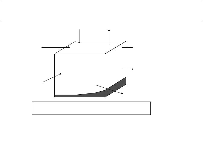
The construction of a mass balance model follows the general outline of this chapter. First, one defines the spatial and temporal scales to be considered and establishes the environmental compartments or control volumes. Second, the source emissions are identified and quantified. Third, the mathematical expressions for advective and diffusive transport processes are written. And last, chemical transformation processes are quantified. This model-building process is illustrated in Figure 27.4. In this example we simply equate the change in chemical inventory (total mass in the system) with the difference between chemical inputs and outputs to the system. The inputs could include numerous point and nonpoint sources or could be a single estimate of total chemical load to the system. The outputs include all of the loss mechanisms: transport
Atmospheric |
Diffusion to |
deposition, Iair |
atomosphere, Oair |
Advective input from river, Iriver
Waste discharges, Iwastes
Homogeneous advection, Odissolved
Environmental compartment
Control voulme, V Concentration, C
Heterogeneous advection, Oparticle
Sedimentation, Osed
Irreversible reaction, Orx
Inventory change = inputs (I) – outputs (O)
Vdc/dt = (Iair + Iriver + Iwastes) – (Oair + Osed + Odissolved + Oparticle + Orx)
at steady state, dc/dt = 0 and (Iair + Iriver + Iwastes) = (Oair + Osed + Odissolved + Oparticle + Orx)
Figure 27.4 A simple chemical mass balance model.
498 TRANSPORT AND FATE OF TOXICANTS IN THE ENVIRONMENT
|
|
Total input = 171 kg/y |
|
|
|
|
|
|
|
|
|
Total loss = 198 kg/y |
||||||
|
|
|
Net removal = 27 kg/y |
|
||||||||||||||
|
|
|
|
|
|
|
|
|
|
|
|
|||||||
Atomospheric deposition |
|
|
|
|
|
|
|
|
|
Loss |
||||||||
|
|
|
|
|
|
|
|
|
||||||||||
|
|
|
|
|
|
|
|
|
processes |
|||||||||
|
|
|
|
|
|
|
|
|
|
|
|
|
|
|
||||
|
64 kg/y |
|
|
|
|
|
|
|
|
|
||||||||
|
|
|
|
|
|
|
|
|
|
|
|
|
3 kg/y |
|||||
|
Boston harbor |
|
|
|
|
Water column (2 kg) |
|
|
|
|||||||||
|
|
|
|
|
|
|
|
|
|
|||||||||
|
75 kg/y |
|
|
|
|
|
|
|
|
|
||||||||
|
|
|
|
|
|
|
|
|
|
|
|
|
|
|
|
|
||
|
Other coastal |
|
|
|
|
|
|
|
|
|
|
|
|
|
|
|
|
|
|
|
2 kg/y |
|
|
|
|
|
|
|
|
|
|
|
|
|
|
|
|
Merrimack river |
|
|
|
Particle |
|
|
|
|
|
|
|
Outflow |
||||||
|
|
|
|
|
|
|
|
|
|
|||||||||
|
30 kg/y |
|
|
|
|
|
|
|
|
|
|
|
|
|||||
|
|
|
|
recycling? |
|
|
|
|
|
|
|
25 kg/y |
||||||
|
|
|
|
|
|
|
|
|
|
|
|
|
||||||
|
|
|
|
|
|
|
|
|
|
|
|
|
|
Desorption? |
|
|
||
|
|
|
|
|
|
|
|
|
|
|
|
|
|
|
|
|
|
|
|
|
|
|
|
|
|
|
|
|
|
|
|
|
|
|
|
|
|
|
|
|
|
|
|
Burial |
|
|
Surface sediment (2,400 kg) |
|
|
|||||||
|
|
|
|
|
|
170 kg/y |
|
|
Total sediment (14,500 kg) |
|
|
|||||||
|
|
|
|
|
|
|
|
|
||||||||||
|
|
|
|
|
|
|
|
|
|
|
|
|
|
|
|
|
|
|
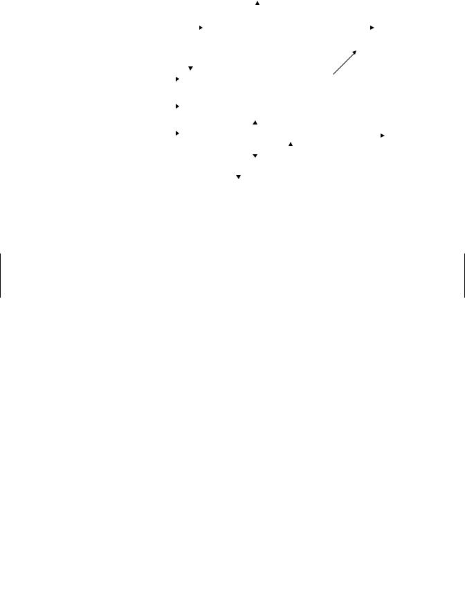
Mass Budget for Benzo(a)pyrene
Figure 27.5 Information provided by a chemical mass balance model. The annual mass budget of benzo[a]pyrene in Massachusetts Bay is shown.
out of the compartment and irreversible transformation reactions. If steady state can be assumed (i.e., the chemical’s concentration in the compartment is not changing over the time scale of the model), the inventory change is zero and we are left with a simple mass balance equation to solve. Unsteady-state conditions would require a numerical solution to the differential equations.
There are many tricks and shortcuts to this process. For example, rather than compiling all of the transformation rate equations (or conducting the actual kinetic experiments yourself), there are many sources of typical chemical half-lives based on pseudo-first- order rate expressions. It is usually prudent to begin with these “best estimates” of half-lives in air, water, soil, and sediment and perform a sensitivity analysis with the model to determine which processes are most important. One can return to the most important processes to assess whether more detailed rate expressions are necessary. An illustration of this mass balance approach is given in Figure 27.5 for benzo[a]pyrene. This approach allows a first-order evaluation of how chemicals enter the environment, what happens to them in the environment, and what the exposure concentrations will be in various environmental media. Thus the chemical mass balance provides information relevant to toxicant exposure to both humans and wildlife.
SUGGESTED READING
Hemond, H. F., and E. J. Fechner. Chemical Fate and Transport in the Environment. New York: Academic Press, 1994.
Mackay, D., W. Y. Shiu, and K. C. Ma. Physical-Chemical Properties and Environmental Fate and Degradation Handbook. CRCnetBASE 2000 CR-ROM. Boca Raton, FL: CRC Press, 2000.

SUGGESTED READING |
499 |
Mackay, D. Multimedia Environmental Models: The Fugacity Approach, 2nd ed. Boca Raton, FL: Lewis Publishers, 2001.
Rand, G. M., ed. Fundamentals of Aquatic Toxicology: Part II Environmental Fate. Washington, DC: Taylor and Francis, 1995.
Schnoor, J. L. Environmental Modeling: Fate and Transport of Pollutants in Water, Air, and Soil. New York: Wiley, 1996.
Schwarzenbach, R. P., P. M. Gschwend, and D. M. Imboden. Environmental Organic Chemistry, 2nd ed. New York: Wiley, 2002.
- #15.08.20134.04 Mб15Hastie T., Tibshirani R., Friedman J. - The Elements of Statistical Learning Data Mining, Inference and Prediction (2002)(en).djvu
- #
- #
- #
- #
- #
- #
- #
- #15.08.201315.44 Mб23Hudlicky M, Pavlath A.E. (eds.) - Chemistry of Organic Fluorine Compounds 2[c] A critical Review (1995)(en).djvu
- #
- #