Fitts D.D. - Principles of Quantum Mechanics[c] As Applied to Chemistry and Chemical Physics (1999)(en)

9:274 02 3 10ÿ24 JTÿ1

152	Angular momentum

ing current I enclosing a small area A gives rise to a magnetic moment M of magnitude M given by

M IA

(5:79)

The area A enclosed by the circular electronic orbit of radius r is ðr2. From equation (5.63) we have the relation L meùr2. Thus, the magnitude of the magnetic moment is related to the magnitude L of the angular momentum by

M	eL	(5:80)
	2me

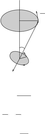
The direction of the vector L is determined by equation (5.62). By convention, the direction of the current I is opposite to the direction of rotation of the negatively charged electron, i.e., opposite to the direction of the vector v. Consequently, the vector M points in the opposite direction from L (see Figure 5.4) and equation (5.80) in vector form is

M		ÿe	L		ÿìB	L	(5:81)
					"
		2me

Since the units of L are those of ", we have de®ned in equation (5.81) the Bohr magneton ìB as

e"

ìB 2me (5:82) The relationship (equation (5.81)) between M and L depends only on fundamental constants, the electronic mass and charge, and does not depend on any of the variables used in the derivation. Although this equation was obtained by applying classical theory to a circular orbit, it is more generally valid. It applies to elliptical orbits as well as to classical motion with attractive forces other than rÿ2 dependence. For any orbit in any central force ®eld, the angular

L

v

A r

I

M

Figure 5.4 The magnetic moment M and the orbital angular momentum L of an electron in a circular orbit.

5.5 Magnetic moment

153

momentum is conserved and, since equation (5.81) applies, the magnetic moment is constant in both magnitude and direction. Moreover, equation (5.81) is also valid for orbital motion in quantum mechanics.

Interaction with a magnetic ®eld

The potential energy V of an atom with a magnetic moment M in a magnetic ®eld B is

V ÿM : B ÿMB cos è

(5:83)

where è is the angle between M and B. The force F acting on the atom due to the magnetic ®eld is

F ÿ=V
or
Fx ÿM :	@B			ÿM cos è	@B
	@x				@x
Fy ÿM :	@B			ÿM cos è	@B	(5:84)
	@ y				@ y
Fz ÿM :	@B			ÿM cos è	@B
	@z				@z

If the magnetic ®eld is uniform, then the partial derivatives of B vanish and the force on the atom is zero.

According to electrodynamics, the force F for a non-uniform magnetic ®eld

produces on the atom a torque T given by
T M 3 B ÿ	ìB	L 3 B	(5:85)
	"

where equation (5.81) has been introduced as well. From the relation T dL=dt in equation (5.6), we have

dL		ÿ	ìB	L 3 B	(5:86)
dt			"

Thus, the torque changes the direction of the angular momentum vector L and the vector dL=dt is perpendicular to both L and B, as shown in Figure 5.5. As a result of this torque, the vector L precesses around the direction of the magnetic ®eld B with a constant angular velocity ùL. This motion is known as Larmor precession and the angular velocity ùL is called the Larmor frequency. Since the magnetic moment M is antiparallel to the angular moment L, it also precesses about the magnetic ®eld vector B.

From equation (5.61), the Larmor angular frequency or velocity ùL is equal to the velocity of the end of the vector L divided by the radius of the circular path shown in Figure 5.5

(5:87)

154	Angular momentum

B

dL

dt

Lsinè

L

è

v

r

I

M

Figure 5.5 The motion in a magnetic ®eld B of the orbital angular momentum vector L.

jdL=dtj

ùL L sin è

The magnitude of the vector dL=dt is obtained from equation (5.86) as

dL ì"B LB sin è dt

so that

ùL ìB"B

If we take the z-axis of the coordinate system parallel to the magnetic ®eld vector B, then the projection of L on B is Lz and cos è in equation (5.83) is

cos è

Lz

l

L

are m

withp•••••••••••••••• . . .

0, 1, . . . and the only allowed values of Lz

In quantum mechanics, the only allowed values of

L

are

l(l 1) "

with

"

m

0,

1,

,

l. Accordingly, the angle è is quantized, being restricted to values for which

The

m

L

B

possiblep••••••••••••••••

,

. . . ,

(5:88)

cos è

l(l 1)

l 0, 1, 2,

m 0, 1, . . . , l

orientations

of

with

respect

to

for the

case l

3

are

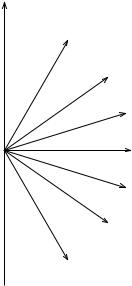
illustrated in Figure 5.6. Classically, all values between 0 and ð are allowed for the angle è. When equations (5.81) and (5.88) are substituted into (5.83), we ®nd that the potential energy V is also quantized

V mìB B, m 0, 1, . . . , l (5:89)

Problems		155
B
m 5 3
	m 5 2
	m 5 1
	m 5 0
	m 5	21
	m 5 22
m 5 23

Figure 5.6 Possible orientations in a magnetic ®eld B of the orbital angular momentum vector L for the case l 3

Problems

	5.1			^	^	^
		Show that each of the operators Lx,			Ly,	Lz is hermitian.
	5.2	Evaluate the following commutators:
		^	^	(c)	^		^	^py]
		(a) [Lx, x]	(b) [Lx, ^px]		[Lx, y]		(d) [Lx,		^
	5.3	Using the commutation relation (5.10b), ®nd the expectation value of								for a
									Lx

system in state jlmi.

5.4					^	^	to obtain an expres-
	Apply the uncertainty principle to the operators Lx					and Ly
	^	^		Evaluate the expression for a system in state					lm		.
	sion for ÄLxÄ	L	y.					j		i
5.5				^2	^	^
	Show that the operator J				commutes with J x and with J y.

5.6Show that J^ and J^ÿ as de®ned by equations (5.18) are adjoints of each other.

5.7Prove the relationships (5.19a)±(5.19g).

5.8Show that the choice for cÿ in equation (5.24) is consistent with c in equation (5.22).

5.9		^	^
	Using the raising and lowering operators J and J ÿ, show that
	^	^
	hjmjJ xjjmi hjmjJ yjjmi 0
5.10	Show that
	hjmjJ^2xjjmi hjmjJ^2yjjmi 21[ j( j 1) ÿ m2]"2
5.11	Show that jj, mi are eigenfunctions	^	^	^ ^
		of [J x, J ] and of		[J y, J ]. Find the

eigenvalues of each of these commutators.

6

The hydrogen atom

A theoretical understanding of the structure and behavior of the hydrogen atom is essential to the ®elds of physics and chemistry. As the simplest atomic system, hydrogen must be understood before one can proceed to the treatment of more complex atoms, molecules, and atomic and molecular aggregates. The hydrogen atom is one of the few examples for which the SchroÈdinger equation can be solved exactly to obtain its wave functions and energy levels. The resulting agreement between theoretically derived and experimental quantities serves as con®rmation of the applicability of quantum mechanics to a real chemical system. Further, the results of the quantum-mechanical treatment of atomic hydrogen are often used as the basis for approximate treatments of more complex atoms and molecules, for which the SchroÈdinger equation cannot be solved.

The study of the hydrogen atom also played an important role in the development of quantum theory. The Lyman, Balmer, and Paschen series of spectral lines observed in incandescent atomic hydrogen were found to obey the empirical equation

		n12		ÿ n22
í		Rc	1	1	,	n2 . n1

where í is the frequency of a spectral line, c is the speed of light, n1 1, 2, 3 for the Lyman, Balmer, and Paschen series, respectively, n2 is an integer determining the various lines in a given series, and R is the so-called Rydberg constant, which has the same value for each of the series. Neither the existence of these spectral lines nor the formula which describes them could be explained by classical theory. In 1913, N. Bohr postulated that the electron in a hydrogen atom revolves about the nucleus in a circular orbit with an angular momentum that is quantized. He then applied Newtonian mechanics to the electronic motion and obtained quantized energy levels and quantized orbital radii. From

156

6.1 Two-particle problem

157

the Planck relation ÄE En1 ÿ En2 hí, Bohr was able to reproduce the experimental spectral lines and obtain a theoretical value for the Rydberg constant that agrees exactly with the experimentally determined value. Further investigations, however, showed that the Bohr model is not an accurate representation of the hydrogen-atom structure, even though it gives the correct formula for the energy levels, and led eventually to SchroÈdinger's wave mechanics. SchroÈdinger also used the hydrogen atom to illustrate his new theory.

6.1 Two-particle problem

In order to apply quantum-mechanical theory to the hydrogen atom, we ®rst need to ®nd the appropriate Hamiltonian operator and SchroÈdinger equation. As preparation for establishing the Hamiltonian operator, we consider a classical system of two interacting point particles with masses m1 and m2 and instantaneous positions r1 and r2 as shown in Figure 6.1. In terms of their

cartesian components, these position vectors are
	r1 ix1 jy1 kz1
	r2 ix2 jy2 kz2
The vector distance between the particles is designated by r
r r2 ÿ r1 ix jy kz			(6:1)
where
x x2 ÿ x1,	y y2 ÿ y1,	z z2 ÿ z1

The center of mass of the two-particle system is located by the vector R with cartesian components, X, Y, Z

z

	2
		CM
	r2	1
	R
		r1
		y

x

Figure 6.1 The center of mass (CM) of a two-particle system.

(6:3)

158 The hydrogen atom

R iX jY k Z

By de®nition, the center of mass is related to r1 and r2 by

	R		m1r1 m2r2	(6:2)
			M

where M m1 m2 is the total mass of the system. We may express r1 and r2 in terms of R and r using equations (6.1) and (6.2)

r1 R ÿ mM2 r r2 R mM1 r

If we restrict our interest to systems for which the potential energy V is a function only of the relative position vector r, then the classical Hamiltonian

function H is given by

H

jp1j2

jp2j2

V(r)

(6:4)

2m1

2m2

where the momenta p1 and p2 for the two particles are

p1 m1

dr1

p2 m2

dr2

,

dt

dt

These momenta may be expressed in terms of the time derivatives of R and r by substitution of equation (6.3)

dR

m2 dr

p1 m1

ÿ

dt

M dt

(6:5)

dR

m dr

p2 m2

1

dt

M

dt

Substitution of equation (6.5) into (6.4) yields

H

21M

dR

2

dr

2

(6:6)

dt

21ì dt

V (r)

where the cross terms have canceled out and

we have de®ned the reduced mass

ì by

ì

m1 m2

m1 m2

(6:7)

m1 m2

M

The momenta pR and pr, corresponding to the center of mass position R and the relative position variable r, respectively, may be de®ned as

pR M	dR	,	pr ì	dr
	dt			dt

In terms of these momenta, the classical Hamiltonian becomes

	6.1	Two-particle problem					159
	H		jpRj2	jprj2		V(r)	(6:8)
			2M	2ì

We see that the kinetic energy contribution to the Hamiltonian is the sum of two parts, the kinetic energy due to the translational motion of the center of mass of the system as a whole and the kinetic energy due to the relative motion of the two particles. Since the potential energy V(r) is assumed to be a function only of the relative position coordinate r, the motion of the center of mass of the system is unaffected by the potential energy.

The quantum-mechanical Hamiltonian operator ^ is obtained by replacing

H

jpRj2 and jprj2 in equation (6.8) by the operators ÿ"2=2R and ÿ"2=2r, respectively, where

@2

@2

@2

=2R

(6:9a)

@X 2

@Y 2

@ Z2

@2

@2

@2

=2r

(6:9b)

@x2

@ y2

@z2

The resulting SchroÈdinger equation is, then,

"ÿ

"2

=2R ÿ

"2

=2r V (r)#Ø(R, r) EØ(R, r)

(6:10)

2M

2ì

This partial differential equation may be readily separated by writing the wave function Ø(R, r) as the product of two functions, one a function only of the center of mass variables X, Y, Z and the other a function only of the relative coordinates x, y, z

Ø(R, r) ÷(X , Y , Z)ø(x, y, z) ÷(R)ø(r)

With this substitution, equation (6.10) separates into two independent partial

differential equations
	ÿ				"2	=2R÷(R) ER÷(R)	(6:11)
				2M
	"2		2		ø(r) V(r)ø(r) Erø(r)
ÿ		=r					(6:12)
	2ì

where

E ER Er

Equation (6.11) is the SchroÈdinger equation for the translational motion of a free particle of mass M, while equation (6.12) is the SchroÈdinger equation for a hypothetical particle of mass ì moving in a potential ®eld V(r). Since the energy ER of the translational motion is a positive constant (ER > 0), the solutions of equation (6.11) are not relevant to the structure of the two-particle system and we do not consider this equation any further.

160 The hydrogen atom

6.2 The hydrogen-like atom

The SchroÈdinger equation (6.12) for the relative motion of a two-particle system is applicable to the hydrogen-like atom, which consists of a nucleus of charge Ze and an electron of charge ÿe. The differential equation applies to H for Z 1, He for Z 2, Li2 for Z 3, and so forth. The potential energy V (r) of the interaction between the nucleus and the electron is a function of their separation distance r jrj (x2 y2 z2)1=2 and is given by Coulomb's law (equation (5.76)), which in SI units is

Ze2 V (r) ÿ 4ðå0 r

where meter is the unit of length, joule is the unit of energy, coulomb is the unit of charge, and å0 is the permittivity of free space. Another system of units, used often in the older literature and occasionally in recent literature, is the CGS gaussian system, in which Coulomb's law is written as

V (r) ÿ Zer 2

In this system, centimeter is the unit of length, erg is the unit of energy, and statcoulomb (also called the electrostatic unit or esu) is the unit of charge. In this book we accommodate both systems of units and write Coulomb's law in the form

V(r) ÿ	Ze92	(6:13)
	r

where e9 e for CGS units or e9 e=(4ðå0)1=2 for SI units.

Equation (6.12) cannot be solved analytically when expressed in the cartesian coordinates x, y, z, but can be solved when expressed in spherical polar coordinates r, è, j, by means of the transformation equations (5.29). The laplacian operator =2r in spherical polar coordinates is given by equation (A.61) and may be obtained by substituting equations (5.30) into (6.9b) to yield

1 @

@

1

1

@

@

1 @2

=2r

r2

@r

r2

@r

r2

"

sin è

@è

sin è

@è

sin2 è

@j2

#

If this expression is compared with equation (5.32), we see that

1 @

@

1

=2r

r2

ÿ

^L2

r2

@r

@ r

"2 r2

where ^2 is the square of the orbital angular momentum operator. With the

L

laplacian operator =2r expressed in spherical polar coordinates, the SchroÈdinger equation (6.12) becomes

6.3 The radial equation

161

^

j)

with

Hø(r, è, j) Eø(r, è,

r2

H^ ÿ

"2

@

@

1

^L2 V(r)

(6:14)

2ìr2

@r

@r

2ìr2

^2

in equation (5.32) commutes with the Hamiltonian operator

The operator L

^

^2

H in (6.14) because L commutes with itself and does not involve the variable

r. Likewise, the operator

^

^

because it

Lz

in equation (5.31c) commutes with H

^2

as shown in (5.15a) and also does not involve the variable r.

commutes with L

Thus, we have

^

,

^2

0,

^

^

^2

^

[H

L ]

^

[ H,

Lz] 0,

[L ,

Lz] 0

and the operators

^ ^2

H, L , and

Lz have simultaneous eigenfunctions,

^

ø(r, è, j) Eø(r,

è, j)

(6:15a)

H

^2

2

ø(r, è, j),

l 0, 1, 2, . . .

(6:15b)

L

ø(r, è, j) l(l 1)"

^

ø(r, è, j) m"ø(r, è, j),

m ÿl, ÿl 1, . . . , l ÿ 1,

l (6:15c)

Lz

^2

^

are the spherical harmonics

The simultaneous eigenfunctions of L

and Lz

^2

^

Ylm(è, j) given by equations (5.50) and (5.59). Since neither L nor Lz involve

the variable r, any speci®c spherical harmonic may be multiplied by an arbitrary function of r and the result is still an eigenfunction. Thus, we may write ø(r, è, j) as

ø(r, è, j) R(r)Ylm(è, j)

(6:16)

Substitution of equations (6.13), (6.14), (6.15b), and (6.16) into (6.15a) gives

		^		R(r) ER(r)				(6:17)
where		Hl
	"2		d		d		Ze92
H^ l ÿ				r2		ÿ l(l 1) ÿ		(6:18)
	2ìr2		dr		dr		r

and where the common factor Ylm(è, j) has been divided out.

6.3 The radial equation

Our next task is to solve the radial equation (6.17) to obtain the radial function R(r) and the energy E. The many solutions of the differential equation (6.17) depend not only on the value of l, but also on the value of E. Therefore, the solutions are designated as REl(r). Since the potential energy ÿZe92=r is always negative, we are interested in solutions with negative total energy, i.e., where E < 0. It is customary to require that the functions REl(r) be normal-