Fitts D.D. - Principles of Quantum Mechanics[c] As Applied to Chemistry and Chemical Physics (1999)(en)

182		The hydrogen atom
z			z
2	1	2	1

		x				y
1	2		1		2
	3dxz				3dyz
	y
2	1
		x
1	2
	3dxy
				z
	y
	2		1
1		1
			2	2		any axis '
						z-axis
			x
	2		1

3dx22y2

3dz2

Figure 6.3 Polar graphs of the hydrogen 3d atomic orbitals. Regions of positive and negative values of the orbitals are indicated by and ÿ signs, respectively. The distance of the curve from the origin is proportional to the square of the angular part of the atomic orbital.

6.4 Atomic orbitals

183

aì3/2R10 2

1.5

1

0.5

0	1	2	3	4	r/aì
0					5

aì3/2R2l 0.8
0.6
0.4	l 5 0
0.2			l 5 1
0
20.2	2	4	6	8	r/aì
0					10

aì3/2R3l 0.4
0.3
0.2	l 5 0
0.1		l 5 1		l 5 2
0.0
20.1	2	4	6	8	10	12	14	16	18	r/aì
0										20

Figure 6.4 The radial functions Rnl(r) for the hydrogen-like atom.

184 The hydrogen atom

Z

3

D10(r)

4

r2eÿ2 Zr=a0

a0

1

Z

3

Zr

2

D20(r)

r2

2 ÿ

eÿ Zr=a0

(6:66)

8

a0

a0

1

Z

5

D21(r)

r4eÿ Zr=a0

24

a0

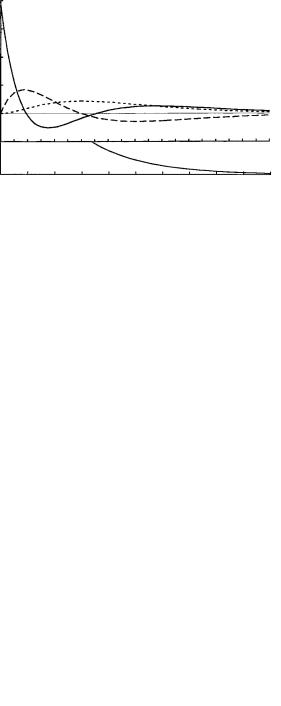
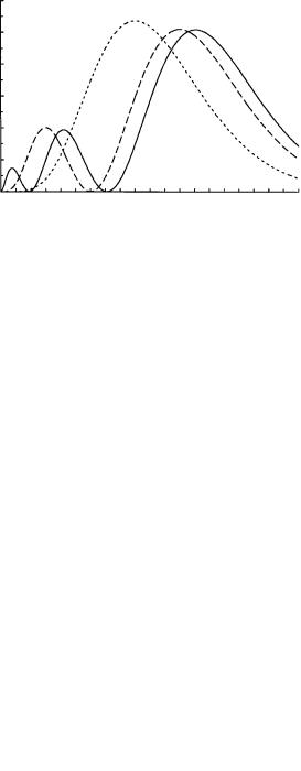
Higher-order functions are readily determined from Table 6.1. The radial distribution functions for the 1s, 2s, 2p, 3s, 3p, and 3d states are shown in Figure 6.5.

The most probable value rmp of r for the 1s state is found by setting the

derivative of D10(r) equal to zero
	dD10(r)		8	Z		3	r 1 ÿ	Zr	eÿ2 Zr=a0	0
	dr			a0				a0
which gives
				rmp a0=Z						(6:67)

Thus, for the hydrogen atom (Z 1) the most probable distance of the electron from the nucleus is equal to the radius of the ®rst Bohr orbit.

The radial distribution functions may be used to calculate expectation values of functions of the radial variable r. For example, the average distance of the electron from the nucleus for the 1s state is given by

1		Z	3	1		3a
hri1s …0	rD10(r) dr 4			…0	r3eÿ2 Zr=a0 dr	0	(6:68)
		a0				2Z

where equations (A.26) and (A.28) were used to evaluate the integral. By the same method, we ®nd

hri2s	6a0	,	hri2p	5a0
	Z			Z

The expectation values of powers and inverse powers of r for any arbitrary state of the hydrogen-like atom are de®ned by

1	1
hrk inl …0	rk Dnl(r) dr …0	rk [Rnl(r)]2 r2 dr	(6:69)

In Appendix H we show that these expectation values obey the recurrence

relation

k 1

rk

(2k

1)

a0

r kÿ1

k l(l

1)

1 ÿ k2

a02

r kÿ2

0

n2

h

inl ÿ

Z h

inl

4

Z2 h

inl

(6:70)

		6.4	Atomic orbitals							185
a0D10 0.60
0.50
0.40
0.30
0.20
0.10
0.00	2	4	6	8	10	12	14	16	18	r/a0
0										20

a0D2l 0.20
0.15
0.10
0.05
0.10					D20
				D21
0.00	2	4	6	8	10	12	14	16	18	r/a0
0										20

a0D3l 0.12
0.10
0.08
0.06
0.04										D30
0.02										D31
0.00										D32
	2	4	6	8	10	12	14	16	18	r/a0
0										20

Figure 6.5 The radial distribution functions Dnl(r) for the hydrogen-like atom.

186

The hydrogen atom

For k 0, equation (6.70) gives

Z

hrÿ1inl

(6:71)

n2 a0

For k 1, equation (6.70) gives

a02

2

r

3a0

l(l

1)

rÿ1

0

n2 h

inl ÿ

Z

Z2 h

inl

or

hrinl

a0

[3n2 ÿ l(l

1)]

(6:72)

2Z

For k 2, equation (6.70) gives

a02

3

hr

2

inl ÿ

5a0

hrinl 2[l(l

1) ÿ

3

0

4]

n2

Z

Z2

or

n2 a2

hr2inl

0

[5n2 ÿ 3l(l 1) 1]

(6:73)

2Z2

For higher values of k, equation (6.70) leads to hr3inl, hr4inl, . . .

For k ÿ1, equation (6.70) relates hrÿ3inl

to hrÿ2inl

hrÿ3inl

Z

hrÿ2inl

(6:74)

l(l

1)a

0

For k ÿ2, ÿ3, . . . ,

equation (6.70) gives successively hrÿ4inl, hrÿ5inl, . . .

expressed in terms of hrÿ2inl.

Although the expectation value hrÿ2inl cannot be obtained from equation (6.70), it can be evaluated by regarding the azimuthal quantum number l as the parameter in the Hellmann±Feynman theorem (equation (3.71)). Thus, we

have
				E			^
									H
		@ n						@ l			(6:75)
		@l							@l
where the Hamiltonian operator			^			is given by equation (6.18) and the energy
			H l
										^
levels En by equation (6.57). The derivative @ Hl=@l is just
^						"	2
	@ H l								(2l	1)	(6:76)
	@l					2ìr2

In the derivation of (6.57), the quantum number n is shown to be the value of l plus a positive integer. Accordingly, we have @n=@l 1 and

@En

Z2 e92 @

Z2 e92 @n @

Z2"2

ÿ

nÿ2 ÿ

nÿ2

nÿ3

(6:77)

@l

2a0

@l

2a0

@l

@n

ìa2

0

where aì "2=ìe92 has been replaced by a0 "2=me e92. Substitution of equations (6.76) and (6.77) into (6.75) gives the desired result

6.5 Spectra

187

hrÿ2inl		Z2		(6:78)
	n3(l		1)a2
			2 0

Expression (6.71) for the expectation value of rÿ1 may be used to calculate the average potential energy of the electron in the state jnlmi. The potential

energy V (r) is given by equation (6.13). Its expectation value is
hV inl ÿZe92hrÿ1inl ÿ	Z2 e92		(6:79)
	a0 n2

The result depends only on the principal quantum number n, so we may drop the subscript l. A comparison with equation (6.57) shows that the total energy is equal to one-half of the average potential energy

En 12hVin (6:80) Since the total energy is the sum of the kinetic energy T and the potential energy V, we also have the expression

Tn ÿEn	Z2 e92	(6:81)
	2a0 n2

The relationship En ÿTn (Vn=2) is an example of the quantum-mechani- cal virial theorem.

6.5 Spectra

The theoretical results for the hydrogen-like atom may be related to experimentally measured spectra. Observed spectral lines arise from transitions of the atom from one electronic energy level to another. The frequency í of any given spectral line is given by the Planck relation

í (E2 ÿ E1)=h

where E1 is the lower energy level and E2 the higher one. In an absorption spectrum, the atom absorbs a photon of frequency í and undergoes a transition from a lower to a higher energy level (E1 ! E2). In an emission spectrum, the process is reversed; the transition is from a higher to a lower energy level (E2 ! E1) and a photon is emitted. A spectral line is usually expressed as a wave number í~, de®ned as the reciprocal of the wavelength ë

	í~		1		í				jE2 ÿ E1j	(6:82)
			ë	c					hc

The hydrogen-like atomic energy levels are given in equation (6.48). If n1 and n2 are the principal quantum numbers of the energy levels E1 and E2, respectively, then the wave number of the spectral line is

188 The hydrogen atom

Table 6.3. Rydberg constant for hydrogen-like atoms

Atom	R (cmÿ1)
1H	109 677.58
2H (D)	109 707.42
4He	109 722.26
7Li2	109 728.72
9Be3	109 730.62
1	109 737.31

	1		1
í~ RZ2			ÿ			,		n2 . n1	(6:83)
		n12		n22
where the Rydberg constant R is given by
		R			ìe94				(6:84)
					4ð"3 c

The value of the Rydberg constant varies from one hydrogen-like atom to another because the reduced mass ì is a factor. It is not appropriate here to replace the reduced mass ì by the electronic mass me because the errors caused by this substitution are larger than the uncertainties in the experimental data. The measured values of the Rydberg constants for the atoms 1H, 4He , 7Li2 , and 9 Be3 are listed in Table 6.3. Following the custom of the ®eld of spectroscopy, we express the wave numbers in the unit cmÿ1 rather than the SI unit mÿ1. Also listed in Table 6.3 is the extrapolated value of R for in®nite nuclear mass. The calculated values from equation (6.84) are in agreement with the experimental values within the known number of signi®cant ®gures for the fundamental constants me, e9, and " and the nuclear masses mN . The measured values of R have more signi®cant ®gures than any of the quantities in equation (6.84) except the speed of light c.

The spectrum of hydrogen (Z 1) is divided into a number of series of spectral lines, each series having a particular value for n1. As many as six different series have been observed:

n1 1,		Lyman series	ultraviolet
n1 2,		Balmer series	visible
n1	3,	Paschen series	infrared
n1	4,	Brackett series	infrared
n1	5,	Pfund series	far infrared
n1	6,	Humphreys series very far infrared

Energy (eV)

0

22

24

26

28

210

212

214

6.5 Spectra

189

Continuum			n 5	∞
			n 5 6
		Pfund	n 5	5
			n 5 4
		series
	Brackett
			n 5 3
Paschen	series
series
Balmer			n 5 2
series

n 5 1 Lyman

series

Figure 6.6 Energy levels for the hydrogen atom.

Thus, transitions from the lowest energy level n1 1 to the higher energy levels n2 2, 3, 4, . . . give the Lyman series, transitions from n1 2 to n2 3, 4, 5, . . . give the Balmer series, and so forth. An energy level diagram for the hydrogen atom is shown in Figure 6.6. The transitions corresponding to the spectral lines in the various series are shown as vertical lines between the energy levels.

190	The hydrogen atom

~	∞
í

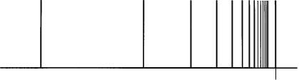
Figure 6.7 A typical series of spectral lines for a hydrogen-like atom shown in terms of the wave number í~.

A typical series of spectral lines is shown schematically in Figure 6.7. The line at the lowest value of the wave number í~ corresponds to the transition n1 ! (n2 n1 1), the next line to n1 ! (n2 n1 2), and so forth. These spectral lines are situated closer and closer together as n2 increases and converge to the series limit, corresponding to n2 1. According to equation (6.83), the series limit is given by

~	R	=	n2	(6 85)
í			1	:

Beyond the series limit is a continuous spectrum corresponding to transitions from the energy level n1 to the continuous range of positive energies for the atom.

The reduced mass of the hydrogen isotope 2H, known as deuterium, slightly differs from that of ordinary hydrogen 1H. Accordingly, the Rydberg constants for hydrogen and for deuterium differ slightly as well. Since naturally occurring hydrogen contains about 0.02% deuterium, each observed spectral line in hydrogen is actually a doublet of closely spaced lines, the one for deuterium much weaker in intensity than the other. This effect of nuclear mass on spectral lines was used by Urey (1932) to prove the existence of deuterium.

Pseudo-Zeeman effect

The in¯uence of an external magnetic ®eld on the spectrum of an atom is known as the Zeeman effect. The magnetic ®eld interacts with the magnetic moments within the atom and causes the atomic spectral lines to split into a number of closely spaced lines. In addition to a magnetic moment due to its orbital motion, an electron also possesses a magnetic moment due to an intrinsic angular momentum called spin. The concept of spin is discussed in Chapter 7. In the discussion here, we consider only the interaction of the external magnetic ®eld with the magnetic moment due to the electronic orbital motion and neglect the effects of electron spin. Thus, the following analysis

6.5 Spectra

191

does not give results that correspond to actual observations. For this reason, we refer to this treatment as the pseudo-Zeeman effect.

When a magnetic ®eld B is applied to a hydrogen-like atom with magnetic moment M, the resulting potential energy V is given by the classical expression

V ÿM : B	ìB	L : B	(6:86)
	"

where equation (5.81) has been introduced. If the z-axis is selected to be parallel to the vector B, then we have

V ìB BLz="

(6:87)

If we replace the z-component of the classical angular momentum in equation

(6.87) by its quantum-mechanical operator, then the Hamiltonian operator					^
					HB
for the hydrogen-like atom in a magnetic ®eld B becomes
^	^	ìB B	^
HB	H	"	Lz	(6:88)

where ^ is the Hamiltonian operator (6.14) for the atom in the absence of the

H

magnetic ®eld. Since the atomic orbitals ønlm in equation (6.56) are simultan-

^	^2		, and		^
eous eigenfunctions of H,	L				Lz, they are also eigenfunctions of the
^
operator H B. Accordingly, we have
H^ Bønlm H^		ìB B		^Lz ønlm (En mìB B)ønlm		(6:89)
			"

where En is given by (6.48) and equation (6.15c) has been used. Thus, the energy levels of a hydrogen-like atom in an external magnetic ®eld depend on the quantum numbers n and m and are given by

	Z2 e92
Enm ÿ	2aì n2 mìB B,	n 1, 2, . . . ; m 0, 1, . . . , (n ÿ 1)

(6:90)

This dependence on m is the reason why m is called the magnetic quantum number.

The degenerate energy levels for the hydrogen atom in the absence of an external magnetic ®eld are split by the magnetic ®eld into a series of closely spaced levels, some of which are non-degenerate while others are still degenerate. For example, the energy level E3 for n 3 is nine-fold degenerate in the absence of a magnetic ®eld. In the magnetic ®eld, this energy level is split into ®ve levels: E3 (triply degenerate), E3 ìB B (doubly degenerate), E3 ÿ ìB B (doubly degenerate), E3 2ìB B (non-degenerate), and E3 ÿ 2ìB B (non-degenerate). Energy levels for s orbitals (l 0) are not affected by the application of the magnetic ®eld. Energies for p orbitals (l 1) are split by the