Fitts D.D. - Principles of Quantum Mechanics[c] As Applied to Chemistry and Chemical Physics (1999)(en)

102	General principles of quantum theory

equivalent procedure. The relation (3.82) is consistent with (1.44), which is based on the Fourier transform properties of wave packets. The difference between the right-hand sides of (1.44) and (3.82) is due to the precise de®nition (3.75) of the uncertainties in equation (3.82).

Similar applications of equation (3.81) using the position±momentum pairs y, ^py and z, ^pz yield

	ÄyÄ py >	"		,	ÄzÄ pz >	"
			2			2

Since x commutes with the operators ^py and ^pz, y commutes with ^px and ^pz, and z commutes with ^px and ^py, the relation (3.81) gives

ÄqiÄ pj 0, i 6 j
where q1 x, q2 y, q3 z, p1 px, p2 py,	p3 pz. Thus, the position
coordinate qi and the momentum component pj	for i 6 j may be precisely
determined simultaneously.

Minimum uncertainty wave packet

The minimum value of the product ÄAÄB occurs for a particular state Ø for which the relation (3.81) becomes an equality, i.e., when

			1	^		^	(3:83)
		ÄAÄB 2jh[A,				B]ij
According to equation (3.79), this equality applies when
	^		^	ÿ hBi)]Ø 0			(3:84)
	[A ÿ hAi ië(B
							^
where ë is given by (3.80). For the position±momentum example where A x
^	ÿi" d=dx, equation (3.84) takes the form
and B
	ÿi" dx		ÿ hpxi Ø ë (x ÿ hxi)Ø
		d			i
for which the solution is
	Ø ceÿ(xÿhxi)2=2ë"eih pxix="						(3:85)

where c is a constant of integration and may be used to normalize Ø. The real constant ë may be shown from equation (3.80) to be

ë	"		2(Äx)2
	2(Ä px)2			"

where the relation ÄxÄ px "=2 has been used, and is observed to be positive. Thus, the state function Ø in equation (3.85) for a particle with minimum position±momentum uncertainty is a wave packet in the form of a plane wave exp[ihpxix="] with wave number k0 hpxi=" multiplied by a gaussian modulating function centered at hxi. Wave packets are discussed in Section

3.11 Heisenberg uncertainty principle

103

1.2. Only the spatial dependence of Ø has been derived in equation (3.85). The state function Ø may also depend on the time through the possible time dependence of the parameters c, ë, hxi, and hpxi.

Energy±time uncertainty principle

We now wish to derive the energy±time uncertainty principle, which is discussed in Section 1.5 and expressed in equation (1.45). We show in Section 1.5 that for a wave packet associated with a free particle moving in the x- direction the product ÄEÄt is equal to the product ÄxÄ px if ÄE and Ät are de®ned appropriately. However, this derivation does not apply to a particle in a potential ®eld.

The position, momentum, and energy are all dynamical quantities and consequently possess quantum-mechanical operators from which expectation values at any given time may be determined. Time, on the other hand, has a unique role in non-relativistic quantum theory as an independent variable; dynamical quantities are functions of time. Thus, the `uncertainty' in time

cannot be related to a range of expectation values.
To obtain the energy-time uncertainty principle for a					particle in a	time-
^			^
independent potential ®eld, we set A equal to H in equation (3.81)
1			^ ^
(ÄE)(ÄB) > 2jh[H, B]ij					^	^
where ÄE is the uncertainty in the energy as de®ned by (3.75) with A						H.
Substitution of equation (3.72) into this expression gives
2			dt
(ÄE)(ÄB) >	"		dhBi		(3:86)
In a short period of time Ät, the change in the expectation					value of B is given

by

ÄB dhdBt i Ät

When this expression is combined with equation (3.86), we obtain the desired

	result
	(ÄE)(Ät) >	"		(3:87)
			2

We see that the energy and time obey an uncertainty relation when Ät is de®ned as the period of time required for the expectation value of B to change by one standard deviation. This de®nition depends on the choice of the dynamical variable B so that Ät is relatively larger or smaller depending on that choice. If dhBi=dt is small so that B changes slowly with time, then the period Ät will be long and the uncertainty in the energy will be small.

104	General principles of quantum theory

Conversely, if B changes rapidly with time, then the period Ät for B to change by one standard deviation will be short and the uncertainty in the energy of the system will be large.

Problems

3.1 Which of the following operators are linear?

(a) p (b) sin (c) ^ (d) ^ xDx Dx x

3.2Demonstrate the validity of the relationships (3.4a) and (3.4b).

3.3Show that

^

^ ^

^

^

^

^

^

^

[A, [B, C]] [B, [C,

A]] [C, [A, B]] 0

^ ^

^

where A, B, and C are arbitrary linear operators.

^

^

^ 2

ÿ x

2

ÿ 1.

3.4

Show that (Dx 2

x)(Dx ÿ x) Dx

2

ÿ 4x2). What is

3.5

Show that xeÿx

is an eigenfunction of the linear operator (D^ x

the eigenvalue?

3.6

^ 2

^ 2

Show that the operator Dx

is hermitian. Is the operator iDx hermitian?

3.7

Show that if the linear operators

^

and

^

do

not commute, the operators

A

B

^^

^ ^

^

^

(AB

BA) and i[A, B] are hermitian.

3.8If the real normalized functions f (r) and g(r) are not orthogonal, show that their sum f (r) g(r) and their difference f (r) ÿ g(r) are orthogonal.

3.9	Consider the set of functions		ø1 eÿx=2,	ø2 xeÿx=2, ø3 x2eÿx=2,		ø4
	x3eÿx=2, de®ned over the range 0 < x < 1. Use the Schmidt orthogonalization
	procedure to construct from the set øi an			orthogonal	set of functions	with
	w(x) 1.
3.10	Evaluate the following commutators:
	(a) [x, ^px]	2	^	^	]
		(b) [x, ^px]	(c) [x, H]	(d) [^px, H

3.11Evaluate [x, ^p3x] and [x2, ^p2x] using equations (3.4).

3.12Using equation (3.4b), show by iteration that

	[x n, ^px] i"nx nÿ1
	where n is a positive integer greater than zero.
3.13	Show that
	[ f (x), ^px] i"	d f (x)
		dx
3.14	Calculate the expectation values of x, x2, ^p, and ^p2 for a particle in a one-
	dimensional box in state øn (see Section 2.5).
3.15	Calculate the expectation value of ^p4 for a particle in a one-dimensional box in
	state øn.
3.16	^
	A hermitian operator A has only three normalized eigenfunctions ø1, ø2, ø3,
	with corresponding eigenvalues a1 1,	a2 2, a3 3, respectively. For		a
	particular state ö of the system, there is a 50% chance that a measure of			A

produces a1 and equal chances for either a2 or a3.

Problems

105

(a)Calculate hAi.

(b)Express the normalized wave function ö of the system in terms of the

	^
	eigenfunctions of A.
3.17	The wave function Ø(x) for a particle in a one-dimensional box of length a is
	Ø(x) C sin7		ðx	; 0 < x < a
			a
	where C is a constant. What are the possible observed values for the energy and
	their respective probabilities?
3.18	If jøi is an eigenfunction of	^	^
		H with eigenvalue E, show that for any operator A
	^	^
	the expectation value of [H,	A] vanishes, i.e.,
		^	^
	høj[ H,		A]jøi 0
3.19	Derive both of the Ehrenfest theorems using equation (3.72).
3.20	Show that

"

ÄHÄx > 2m h^pxi

4

Harmonic oscillator

In this chapter we treat in detail the quantum behavior of the harmonic oscillator. This physical system serves as an excellent example for illustrating the basic principles of quantum mechanics that are presented in Chapter 3. The SchroÈdinger equation for the harmonic oscillator can be solved rigorously and exactly for the energy eigenvalues and eigenstates. The mathematical process for the solution is neither trivial, as is the case for the particle in a box, nor excessively complicated. Moreover, we have the opportunity to introduce the ladder operator technique for solving the eigenvalue problem.

The harmonic oscillator is an important system in the study of physical phenomena in both classical and quantum mechanics. Classically, the harmonic oscillator describes the mechanical behavior of a spring and, by analogy, other phenomena such as the oscillations of charge ¯ow in an electric circuit, the vibrations of sound-wave and light-wave generators, and oscillatory chemical reactions. The quantum-mechanical treatment of the harmonic oscillator may be applied to the vibrations of molecular bonds and has many other applications in quantum physics and ®eld theory.

4.1 Classical treatment

The harmonic oscillator is an idealized one-dimensional physical system in which a single particle of mass m is attracted to the origin by a force F

proportional to the displacement of the particle from the origin
F ÿkx	(4:1)

The proportionality constant k is known as the force constant. The minus sign in equation (4.1) indicates that the force is in the opposite direction to the direction of the displacement. The typical experimental representation of the oscillator consists of a spring with one end stationary and with a mass m

106

ù 2ðí

(4:4)

4.1 Classical treatment

107

attached to the other end. The spring is assumed to obey Hooke's law, that is to say, equation (4.1). The constant k is then often called the spring constant.

In classical mechanics the particle obeys Newton's second law of motion

d2 x
F ma m dt2	(4:2)

where a is the acceleration of the particle and t is the time. The combination of equations (4.1) and (4.2) gives the differential equation

d2 x		ÿ	k
				x
	dt2		m
for which the solution is
x A sin(2ðít b) A sin(ùt b)					(4:3)

where the amplitude A of the vibration and the phase b are the two constants of integration and where the frequency í and the angular frequency ù of

vibration are related to k and m by

r•••• k

m

According to equation (4.3), the particle oscillates sinusoidally about the origin with frequency í and maximum displacement A.

The potential energy V of a particle is related to the force F acting on it by the expression

F ÿ ddVx

Thus, from equations (4.1) and (4.4), we see that for a harmonic oscillator the potential energy is given by

V 21kx2 21mù2 x2

(4:5)

The total energy E of the particle undergoing harmonic motion is given by

E 21 mv2 V 21mv2 21mù2 x2

(4:6)

where v is the instantaneous velocity. If the oscillator is undisturbed by outside forces, the energy E remains ®xed at a constant value. When the particle is at maximum displacement from the origin so that x A, the velocity v is zero and the potential energy is a maximum. As jxj decreases, the potential

decreases and the velocity increases keeping E constant. As the particle crosses
To relate the maximum displacement A to the constant		p•••••••••••••
the origin (x 0), the velocity attains its maximum value v		2E=m.

energy E, we note

that when x A, equation (4.6) becomes

E 12mù2 A2

so that

108	Harmonic oscillator

r••••••

12E

A

ù

m

Thus, equation (4.3) takes the form

ù r••••••

x

1

2E

sin(ùt b)

(4:7)

m

By de®ning a reduced distance y as

r••••••

y

ù

m

x

(4:8)

2E

so that the particle oscillates between y ÿ1 and y 1, we may express the equation of motion (4.7) in a universal form that is independent of the total energy E

y(t) sin(ùt b)		(4:9)
As the particle oscillates back and forth between	y ÿ1 and	y 1, the
probability that it will be observed between some	value y and	y dy is

P( y) dy, where P(y) is the probability density. Since the probability of ®nding the particle within the range ÿ1 < y < 1 is unity (the particle must be some-

where in that range), the probability density is normalized

…1

P(y) d y 1

ÿ1

The probability of ®nding the particle within the interval dy at a given distance y is proportional to the time dt spent in that interval

P( y) dy c dt c ddyt dy

so that

P( y) c ddyt

where c is the proportionality constant. To ®nd P(y), we solve equation (4.9) for t

t(y) ù1 [sinÿ1(y) ÿ b] and then take the derivative to give

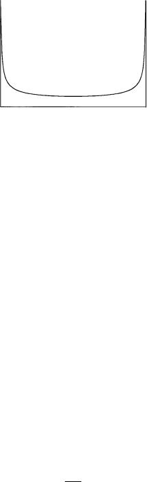
P(y) ùc (1 ÿ y2)ÿ1=2 ð1 (1 ÿ y2)ÿ1=2 (4:10)

where c was determined by the normalization requirement. The probability density P(y) for the oscillating particle is shown in Figure 4.1.

4.2 Quantum treatment

109

P(y)

21

y

1

Figure 4.1 Classical probability density for an oscillating particle.

4.2 Quantum treatment

The classical Hamiltonian H(x,

p) for the harmonic oscillator is

p2

p2

H(x, p)

V(x)

21mù2 x2

(4:11)

2m

2m

The Hamiltonian operator

^

^p) is obtained by replacing the momentum p

H(x,

in equation (4.11) with the momentum operator ^p ÿi" d=dx

^

^p2

1

2

2

"2 d2

2

2

1

H

2mù

x

ÿ

2mù

x

(4:12)

2m

2m

dx2

The SchroÈdinger equation is, then

ÿ

"2 d2ø(x)

21mù2 x2ø(x) Eø(x)

(4:13)

2m

dx2

It is convenient to introduce the dimensionless variable î by the de®nition

î

mù

1=2 x

(4:14)

"

so that the Hamiltonian operator becomes

"ù

2

H^

î2 ÿ

d

(4:15)

2

dî2

Since the Hamiltonian operator is written in terms of the variable î rather than x, we should express the eigenstates in terms of î as well. Accordingly, we de®ne the functions ö(î) by the relation

" 1=4

ö(î) mù ø(x) (4:16)

If the functions ø(x) are normalized with respect to integration over x

110	Harmonic oscillator
	1
	…ÿ1jø(x)j2 dx 1

then from equations (4.14) and (4.16) we see that the functions ö(î) are
normalized with respect to integration over î
	…ÿ1jö(î)j2 dî 1
	1
The SchroÈdinger equation (4.13) then takes the form
ÿ	d2ö(î)	î2ö(î)	2E
	dî2		"ù ö(î)	(4:17)

Since the Hamiltonian operator is hermitian, the energy eigenvalues E are real. There are two procedures available for solving this differential equation. The older procedure is the Frobenius or series solution method. The solution of equation (4.17) by this method is presented in Appendix G. In this chapter we use the more modern ladder operator procedure. Both methods give exactly the

same results.

Ladder operators

We now solve the SchroÈdinger eigenvalue equation for the harmonic oscillator by the so-called factoring method using ladder operators. We introduce the

two ladder operators ^a and ^ay by the de®nitions
^a		mù		1=2		i^p		1		d	(4:18a)
	2"				x mù			p2	î dî
^ay		mù		1=2		i^p		1•••		d	(4:18b)
	2"				x ÿ mù			p2	î ÿ dî
Application of equation (3.33) reveals that the operator a											is the adjoint of a,
								•••	^y		^

which explains the notation. Since the operator ^a is not equal to its adjoint ^ay, neither ^a nor ^ay is hermitian. (We follow here the common practice of using a lower case letter for the harmonic-oscillator ladder operators rather than our usual convention of using capital letters for operators.) We readily observe that

1

d

2

^

1

H

^a^ay

î2

ÿ

1

(4:19a)

2

dî2

"ù

2

1

d

2

^

1

H

^ay^a

î2

ÿ

ÿ 1

ÿ

(4:19b)

2

dî2

"ù

2

from which it follows that the commutator of ^a and ^ay is unity

[^a, ^ay] ^a^ay ÿ ^ay^a 1

(4:20)

We next de®ne the number operator N^ as the product ^ay^a

	4.2 Quantum treatment	111
	N^ ^ay^a	(4:21)
	^
	The adjoint of N may be obtained as follows
	N^ y (^ay^a)y ^ay(^ay)y ^ay^a N^	^
	where the relations (3.40) and (3.37) have been used. We note that
		N is self-

adjoint, making it hermitian and therefore having real eigenvalues. Equation (4.19b) may now be written in the form

			^	^	1	(4:22)
	^	^	H	"ù(N	2)
Since
	H and N differ only by the factor "ù and an additive constant, they
commute and, therefore, have the same eigenfunctions.
If	the	^	are	represented by the		parameter ë and the
		eigenvalues of N

corresponding orthonormal eigenfunctions by öëi(î) or, using Dirac notation, by jëii, then we have

		^			(4:23)
and		Njëii ëjëii
^	^	1	1		(4:24)
Hjëii "ù(N		2)jëii "ù(ë	2)jëii Eëjëii	^
Thus, the energy eigenvalues Eë are related to the eigenvalues of
				N by
The index i in jëii		Eë (ë 21)"ù			(4:25)
	takes on integer values from 1 to gë, where gë				is the

degeneracy of the eigenvalue ë. We shall ®nd shortly that each eigenvalue of ^

N is non-degenerate, but in arriving at a general solution of the eigenvalue equation, we must initially allow for degeneracy.

	^
From equations (4.20) and (4.21), we note that the product of N and either ^a
or ^ay may be expressed as follows
N^ ^a ^ay^^aa (^^aay ÿ 1)^a ^a(^ay^a ÿ 1) ^a(N^ ÿ 1)		(4:26a)
	N^ ^ay ^ay^^aay ^ay(^ay^a 1) ^ay(N^ 1)	(4:26b)
These identities are useful in the following discussion.
	^
If we let the operator N act on the function ^ajëii, we obtain
^	^	(4:27)
N ^ajëii ^a(N ÿ 1)jëii ^a(ë ÿ 1)jëii (ë ÿ 1)^ajëii

where equations (4.23) and (4.26a) have been introduced. Thus, we see that

^jë i is an eigenfunction of ^ with eigenvalue ë ÿ 1. The operator ^ alters the a i N a

eigenstate jë i to an eigenstate of ^ corresponding to a lower value for the i N

eigenvalue, namely ë ÿ 1. The energy of the oscillator is thereby reduced, according to (4.25), by "ù. As a consequence, the operator ^a is called a lowering operator or a destruction operator.

Letting ^ operate on the function ^yjë i gives

N a i